Geodesic distance and area
measurements
|
1. Create a folder called Geodesic_geom somewhere under your personal directory (e.g. C:\Users\jdoe\Documents\Tutorials\Geodesic_geom). 2. Download the data for this exercise and extract the files from the Geodetic_geom.zip file to your newly created Geodesic_geom directory. |
When working at small scales (i.e. large spatial extents), it may prove difficult to find a coordinate system appropriate for distance or area based measurements. This short exercise shows you how to circumvent coordinate system limitations by adopting geodesic based solutions.
Step 1: Selecting
by distance (planar vs geodetic)
Step 2: Calculating polygon surface area (planar vs.
geodetic)
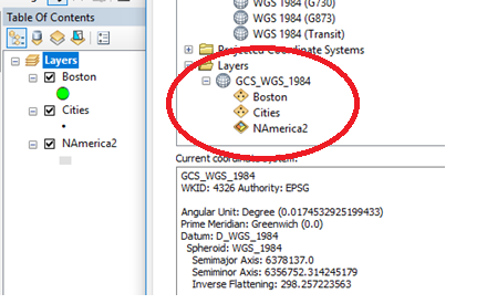
Open the Geodesic_measurements.mxd document from the project folder.
You’ll note from the data frame properties that the coordinate system associated with both the data frame and the three layers is a geographic one (i.e. one defined on an ellipsoid and not on a cartesian coordinate system).
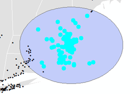
However, ArcMap will not perform geodesic based distance selections when using the Select by Location tool accessed via the Selection pull-down menu (at least with ArcGIS version 10.6 and below). To confirm this, we will first draw a Tissot circle to identify a true 100 mile search radius around the city of Boston.
Open the Geoprocessing >> Buffer tool and create a 100 mile geodesic buffer around the Boston point layer. Name the output Buf100mi.shp.
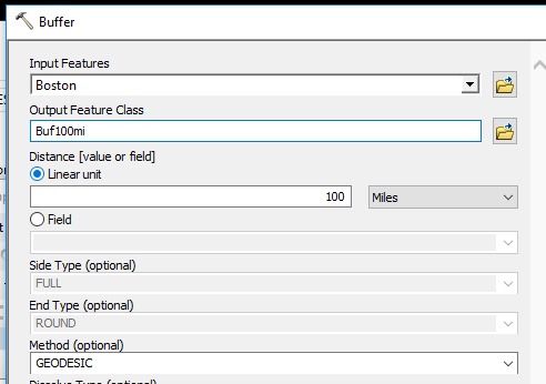
Click OK to run the geoprocess.
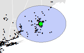
This should generate a true 100 mile circle around the city of Boston. You’ll note the distorted shape in the current reference system. This reflects the distortion associated with the coordinate system ArcMap uses to render a GCS based data frame in the Map View window. ArcMap defaults to a pseudo-plate carrée projection when a GCS defines the data frame.
Next, open the Selection >> Select By Location tool.
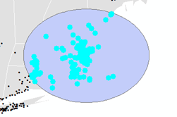
Select all cities that are within 100 miles from Boston.
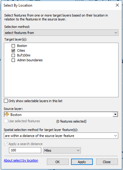
Click OK to run the geoprocess.
You’ll note from the selection that many points inside the geodesic 100 mile buffer are not selected. This confirms that ArcMap defaults to a plate carrée projection when performing a selection in a GSC data frame.
NOTE: The Selection by Location tool used in the
last step inherits the coordinate system associated
with the data frame and not that
associated with the data layer(s) taking part in the selection process. For
example, if the Boston point layer was defined in a projected coordinate system
that preserved distance, the Select by Location tool (accessed via the
Selection pull-down menu) would ignore it and inherit the data frame’s
coordinate system instead.
Next, we’ll perform the same selection using a geodesic distance measurement.
To select the points using a geodesic distance (a better approach), you need to use the Data Management >> Layers and Table Views >> Select Layer By Location tool from the toolbox.
Fill out the fields as
shown below (note the use of the Within_a_distance_geodesic
relationship method).
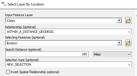
Click OK to run the selection.
Note that now, all points within the geodesic buffer are selected (as expected).
While the Selection by Location tool is readily accessible via the Selection pull-down menu (thus making it a tempting got-to tool), you should only use it when you are certain that the coordinate system adopted by the data frame preserves distance. Otherwise, it may be safer to use the Data Management >> Layers and Table Views >> Select Layer By Location tool with its geodesic measurement option as outlined above.
Geometric calculations such as area are also sensitive to the coordinate system adopted. Therefore, when calculating area (or distance) values in a layer’s attribute table, you must make sure that the coordinate system defining the layer does a good job in preserving area (or distance if calculating distances). If an appropriate coordinate system for the study area is not available you should revert to a geodesic area calculation. In the following examples, we will add two area attribute columns to the Buf100mi layer created in the last step. One of the areas will be computed using the data layer’s GCS and the other using a geodesic area method.
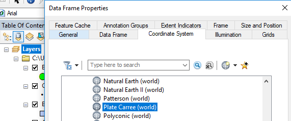
But first, you will change the data frame’s CS to the plate carree projected coordinate system (PCS). The data frame or the data layer must be in a PCS to take advantage of the built-in geometry calculato. Note that the plate carree projection does not do a good job in preserving distance for our study extent as was demonstrated in the last step. This serves only to demonstrate what not to do given our example.
NOTE: In the last step, you were warned that the Selection by Location tool ignored the data layer’s coordinate system and inherited the data frame’s coordinate system instead. However, geometric calculations in an attribute table (such as area and length) allow you to choose either the data frame’s coordinate system or the data layer’s coordinate system. So be mindful of which coordinate system you pick.
Bring up the data frame’s Properties window by double-clicking on the data frame and selecting the Properties tab. Then select the plate carre projection via Projected Coordinate Systems >> World >> Plate Carree.
Right-click the Buf100mi layer and bring up its attribute table.
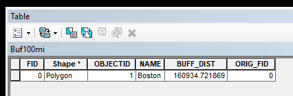
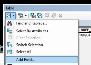
Click on the upper left-hand tab and select Add Field.
Name the field area_PCS and make it a Float type.
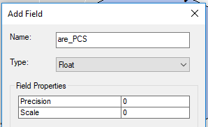
Click OK.
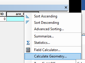
Right-click on the area_PCS field name and select Calculate Geometry. You might be presented with a warning window which you can freely dismiss.
Modify the fields as shown in the following graphic.
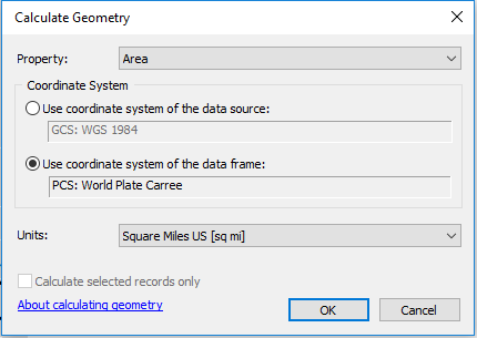
Click OK.
Note that because the data layer (identified as data source in the menu) is in a GCS, its option is ghosted out (the area calculation is only designed for a cartesian CS).
The computed value should be about 42542 mi2.
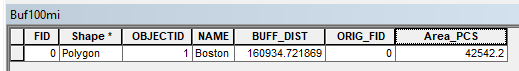
While this area calculation is “correct” in the current coordinate system, it’s not reflective of the true area of the 100 mile radius circle. Recall that the area of a circle is pr2 or 3.145 * 1002 = 31415 mi2 and also recall that we created this buffer using a geodetic method that ensures a correct buffer.
Next, we’ll calculate a geodetic area value making use of a simple Python code.
Create another field and name it area_Geod and make it a Float type.
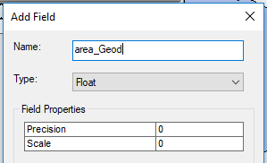
Click OK.
Next, right-click on the area_Geod field name and select Field Calculator.
Check the Python parser option and type the following expression in the expression box:
!Shape!.getArea("Geodesic", "squaremiles").
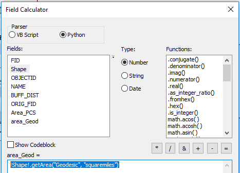
Click OK.
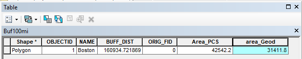
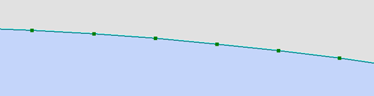
The area value is much closer to what we would expect. The discrepancy is probably due in part to the nature of the circle created from the buffer tool. It’s a non-parametric object meaning the circumference is approximated by small line segments as shown in the following figure.
You can calculate other units using the following parameters: "SQUAREKILOMETERS", "ACRES", “HECTARES” and “SQUAREMETERS”.
Note that you can modify the script to compute line feature geodetic lengths using the following syntax:
!Shape!.getLength("Geodesic", "miles").
© Manny Gimond,