Calculating average income by distance
|
1. Create a folder called Income_dist somewhere under your personal directory (e.g. C:\Users\jdoe\Documents\Tutorials\Income_dist). 2. Download the data for this exercise and extract the files from the Income_dist.zip file to your newly created Income_dist directory. |
In this exercise, you will compute the weighted mean income for various distance bands from Augusta. Geoprocessing tools you will use for the analysis include:
· Buffer (multi-ring buffer)
· Clip
· Intersect
· Dissolve
Step 2: Creating distance bands
Step 3: Computing the distance bands area
Step 4: Intersect distance bands with income
Step 5: Computing weighted income values
Step 6: Dissolving polygons by distance band
Start ArcMap and open Income_dist.mxd from your Income_dist folder.
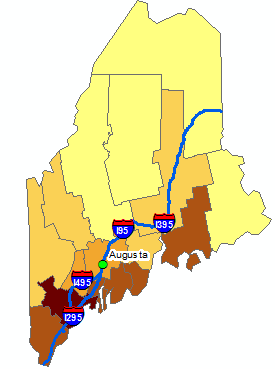
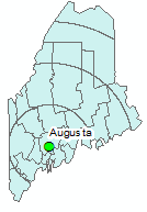
The document consists of three layers: A point layer showing the location of Augusta (the state capital), median per-capita income for 2010 (aggregated at the county level), and the interstate system (used in this exercise as a geographic reference only).
In the following steps, you will create distance bands centered on Augusta, clip the distance bands to the State of Maine then intersect the clipped bands with the income layer. The exercise will finish off by dissolving the intersected polygons by distance then computing the weighted mean income values within each distance band.
You will create distance bands by using one of ArcMap’s buffer tools--the multiple ring buffer tool.
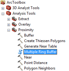
From the Toolbox, select Analysis Tools >> Proximity >> Multiple Ring Buffer.
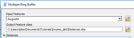
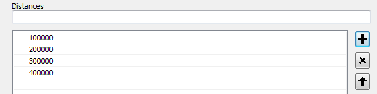
You will select Augusta as the input feature and Distances as the output shapefile.
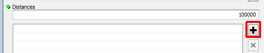
Next, you will specify the distance bands. The first
distance band is 100 km. The tool adopts the map coordinate system’s XY units
(meters in this example) thus the distance will need to be converted to meters.
Type 100000 in the Distances field then click the ![]() icon.
icon.
Add three more distance bands: 200 km, 300 km and 400 km.
Click OK to run the geoprocess.
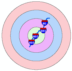
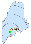
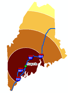
The output should look like a bullseye.
Next, you will clip the distance bands to the State of Maine.
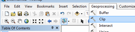
From the pull-down menu select Geoprocessing >> Clip.
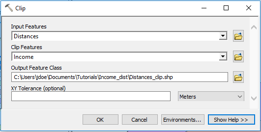
The input layer (layer to be clipped) is Distances and the Clip Features layer is Income. Name the output Distances_clip.
Click OK to run the geoprocess.
Your Distances_clip layer should look like this (you might want to turn off the Distances layer in the TOC):
In the next step, you will create an area field.
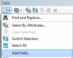
Open the Distances_clip attribute table. Click the top-left icon and select Add Field.
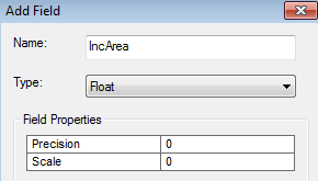
Name the new field Area and set its data type to Float.
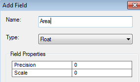
Click OK.
Right-click on the new field and select Calculate Geometry. You might be presented with a window warning you that any calculation made in this session cannot be undone, press Yes to proceed.
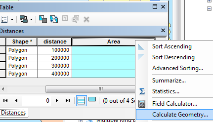
Select Area as the Property type and Square Miles US as the output units.
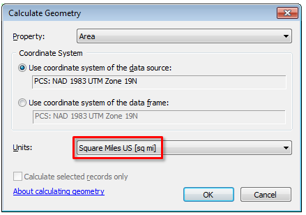
Click OK to run the geoprocess (and Yes if the same warning window pops up).
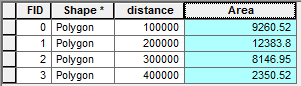
You now have the area (in square miles) for each distance band.
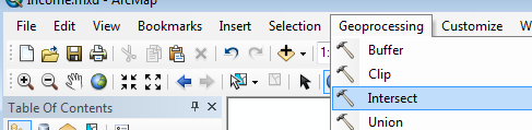
Next, you will combine the Distances_clip layer with the Income layer using the Intersect tool.
Select Geoprocessing >> Intersect.
You will add two layers to the Features table: Income and Distances_clip. Each layer will be added one at a time by selecting it from the Input Features field. Name the output Income_bands.
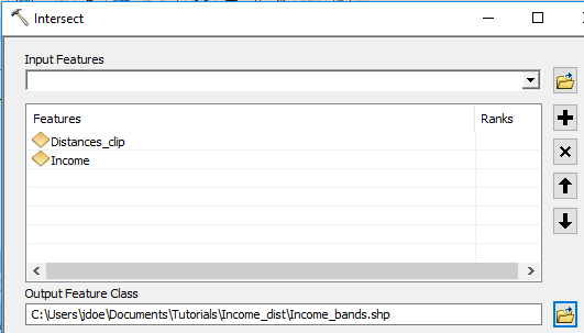
Click OK to run the geoprocess.
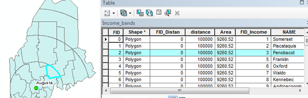
You should see both the counties outline and the bands outline in the new layer.
You will note that the intersection of the two layers created more polygons than the combined input polygons—29 output polygons vs 20 combined input polygons (16 counties + 4 distance bands polygons). This will allow us to recombine the polygons into the original bands later in this exercise.
To confirm that what appears to be split polygons are indeed split polygons select a record in the attributes table by clicking on that row’s grey box and note the selected polygon in the map.
![]()
In the following example, a piece of Penobscot county is selected.
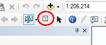
Before moving onto Step 5, make sure to clear any selected features by clicking on the Clear Selected Features icon. If this icon is ghosted out (i.e. inactive), then there are no selected features in your map and you are free to proceed to the next step.
The final step will involve dissolving the polygons into the original distance bands and computing the mean income values within each band. But before we do this, we will need to weigh each income polygon based on its aerial contribution to each distance band.
Open the Income_bands attribute table and create a new field called IncArea (following procedures outlined earlier in this exercise). You will set the data type to Float.
Next, in the IncArea field, calculate the area (in square miles) for each polygon (see Step 3).
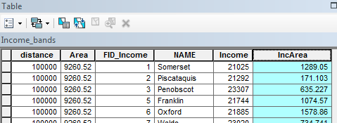
You will use the newly calculate area along with the distance band area (Area field) to compute the weighted income following the formula Income * (IncArea / Area).
In the Income_bands attributes table, create a new field called IncWeight and set its type to Float.
Right-click on the IncWeight field and select Field Calculator. Click Yes if a warning box pops up.
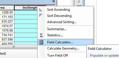
Type the following expression in the expression box: [Income] * ( [IncArea] / [Area]).
![]()
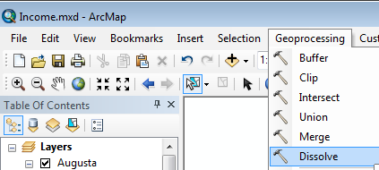
Now each polygon has its weighted income value. In the final step, you will combine all polygons that fall in a common distance bands and sum the weighted income values.
Select Geoprocessing >> Dissolve.
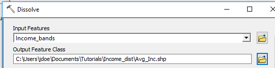
Select Income_bands as the input feature and name the output Avg_Inc.
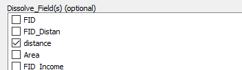
Next, you need to indicate which attribute field will be used to merge contiguous polygons. Since we want to reconstruct the distance bands, we will select the distance field as the dissolve field.
Check the distance layer in the Dissolve_Fields window.
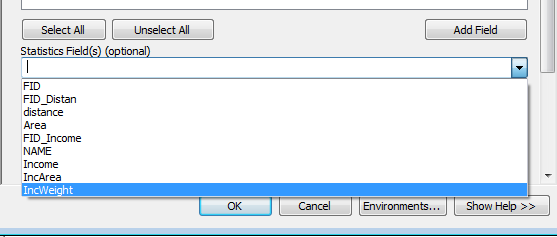
Finally, we will want to instruct ArcMap to sum the weighted income values within each distance band.
In the Statistics field, select IncWeight from the pulldown menu.
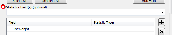
An error symbol will appear next to the Statistics field. This is simply warning us that a Statistics Type has not yet been selected.
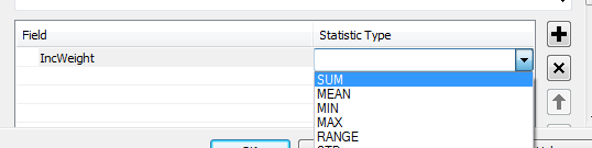
The Statistic Type field allows us to choose which aggregate statistic to use on the dissolved polygons. We will choose to sum the weighted values.
Click on the empty field next to IncWeight and select SUM.
Click OK to run this last geoprocess.
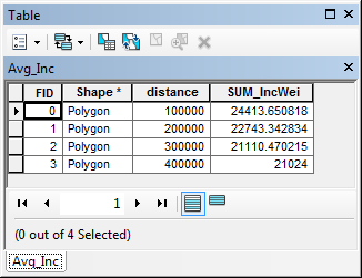
Your final output may not look different from the Distances layer created earlier in this exercise, but if you bring up its attribute table, you’ll see the new column, SUM_IncWei, with the weighted mean income values per distance band.
Symbolize the AVG_Inc layer using the SUM_IncWei column.
This ends this exercise.
![]() Manuel Gimond, last modified on 7/11/2018
Manuel Gimond, last modified on 7/11/2018