Map Algebra: Focal Operations
|
1. Create a folder called MapAlgebraFocal somewhere under your personal directory (e.g. C:\Users\jdoe\Documents\Tutorials\MapAlgebraFocal). 2. Download the MapAlgebraFocal.zip data for this exercise and extract the files to your newly created MapAlgebraFocal directory. |
Note that this tutorial will make use of the Spatial Analyst extension, so make sure to enable this extension from the pull-down menu under Customize >> Extensions. Also, all output files should be saved in the current project folder (i.e. ./MapAlgebraFocal).
Step 2: Smoothing a raster surface: 3 by 3 mean
Step 3: Smoothing a raster surface: 10 km median
Step 4: Smoothing a raster surface: custom neighborhood
Open the Elevation.mxd map document.
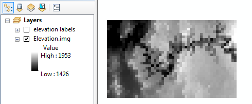
The map consists of an elevation raster (in meters) and a elevation labels layer. The labels layer shows the elevation value for each pixel, but note that this layer is not useful unless you are zoomed in on a subset of pixels.
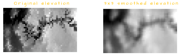
In this step, you will create a new raster where each pixel will reflect the average value of neighboring input pixels. Because the output pixel is influenced by neighboring input pixels (and not just input pixels sharing the same exact location), this type of operation is referred to as a focal operation.
In the following exercise, you will compute the average value from a 3 by 3 cell cluster.
|
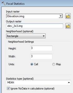
Open the Focal Statistics tool under Spatial Analyst Tools >> Neighborhood.
Set the neighborhood to a 3 cell by 3 cell rectangle and the output statistic to “MEAN”.
Name the output elev_3x3.img. |
|
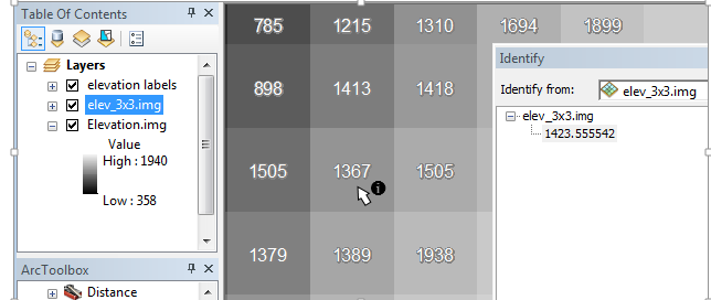
The output raster is made up of the same number of pixels and pixel size as the input layer. The difference is in the raster values.
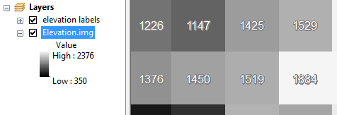
Zoom in on a 3x3 cluster of pixels and extract the pixel value of an elev_3x3.img cell using the Identify tool (make sure to select the elev_3x3.img layer from the identify window). The pixel value should equal the average of the 3x3 cluster.
In the following example, the output cell (selected with the Identify tool) equals (898+1413+1418+1505+1367+1505+1379+1389+1938) / 9 = 1423.56
The Focal Statistics tool can also be used to compute the summary statistic of pixels based on map units and not pixel numbers. In the following example, a 10 km radius is used to define the pixels whose values will be used to compute the output raster pixels. We will also make use of the median as a summary statistic instead of the mean.
|
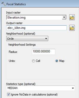
Open the Focal Statistics tool under (under Spatial Analyst Tools >> Neighborhood).
Set the neighborhood to a 10 km (radius) circle and the output statistic to “MEDIAN”.
Name the output elev_10km.img. |
|
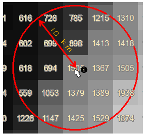
For a pixel to be included in the search radius, its center must fall within the radius. In the following example, pixels whose values are 1310, 1226, 616 and 1874 are not used to compute the output cell at the center of the 10km radius since their centers fall outside of the search radius.
The focal operation does not need to be restricted to a pre-defined list of neighbor definitions, for example, you might want to exclude central cells from the output (i.e. the 3x3 neighbor would consist of 8 input pixels instead of 9).
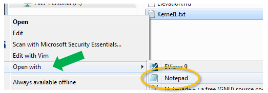
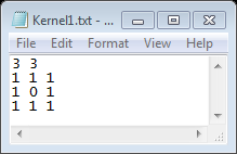
To customize the neighborhood definition, you need to create an ASCII text file. One is already created for this tutorial and is named Kernel1.txt. Note that a text file differs from a Word file and should therefore be created and saved using a basic text editor such as Windows Notepad.
In your project folder, right-click on Kernel1.txt and select to have it opened with Notepad.
The current file consists of 4 lines. The first line defines the width and height of the neighborhood matrix (in pixels) and the next three lines define the neighbor layout with a value of 1 used to define the pixels to include and a value of 0 to define those to exclude
Close the text editor.
Open the Focal Statistics tool (under Spatial Analyst Tools >> Neighborhood). And fill out the first few fields as shown below and select Irregular from the Neighborhood pull-down option.
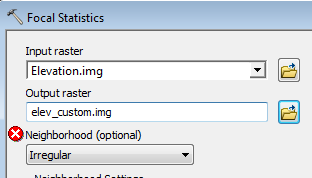
You’ll note that selecting Irregular modifies the tool’s interface.
Select the Kernel1.txt file from your working directory.
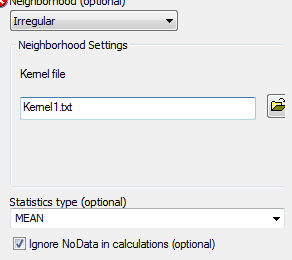
Click OK to run the geoprocess.
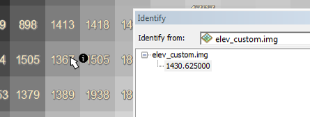
The output values will be different from those in
elev_3x3.img. For example, revisiting the subset of pixels in Step 2, we
compute a slightly different output pixel value of (898+1413+1418+1505+1367+1505+1379+1389+1938) / 8 = 1430.63.
The kernel file can also be used to define cell weights (but note that only the mean, standard deviation and sum statistics can be computed for such a kernel). For example, if we want the right most pixels to be weighted twice as much as the other pixels, the kernel file could look like this:
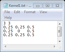
Note that any value can be used (i.e. whole numbers or fractions) as well as both negative and positive numbers.
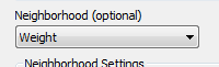
To use a weighted file, you would need to select Weight instead of Irregular from the Neighborhood pulldown option.
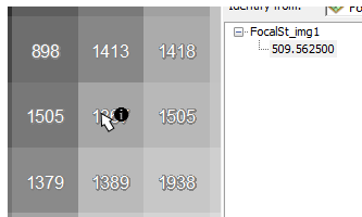
Using the above weight kernel example, the output value for the center of the following cluster of cells would be (898 * .25 + 1413 * .25 + 1418 * .5 + 1505 * .25 + 1505 * .5 + 1379 * .25 + 1389 * .25 + 1938 * .5) / 8 = 509.56.
![]() Manuel Gimond, last
modified on 7/12/2018
Manuel Gimond, last
modified on 7/12/2018