Map Algebra: Local Operations
|
1. Create a folder called MapAlgebraLocal somewhere under your personal directory (e.g. C:\Users\jdoe\Documents\Tutorials\MapAlgebraLocal). 2. Download the MapAlgebraLocal.zip data for this exercise and extract the files to your newly created MapAlgebraLocal directory. |
Note that this tutorial will make use of the Spatial Analyst extension, so make sure to enable this extension from the pull-down menu under Customize >> Extensions. Also, all output files should be saved in the ./MapAlgebraLocal project folder.
Step 2: Create a composite raster of elevation and depth
Step 3: Creating a land/water (binary) raster
Step 4: Extracting the attribute table from integer raster
Step 5: Projecting the raster layer
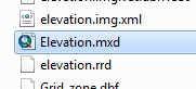
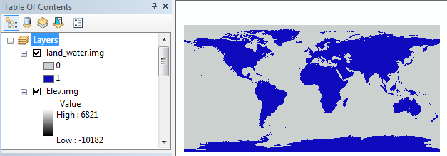
In your MapAlgebraLocal folder, open the Elevation.mxd file.
You should see two layers: a bathymetry layer and an elevation layer.
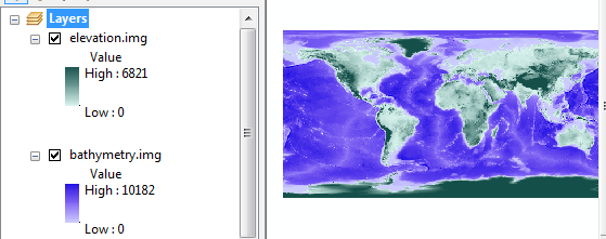
These layers are intended to complement one another (i.e. one shows land based elevation and the other shows ocean based depth).
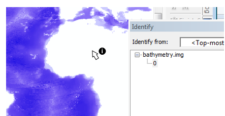
In this step, you will combine both layers into a single one. But first, note that both layers use a pixel value of 0 to denote pixels not covered by the layer. For example, the bathymetry layer has pixel values of 0 for all land based pixels. (Note that you can use the Identify tool to probe pixel values).
Since these rasters complement one another, we can combine them algebraically as we would matrices. However, the bathymetric values are positive downward which is a problem since elevation values are also positive but in the upward direction. So we need to multiply the bathymetry layer by -1 before adding it to the elevation layer. The expression will therefore look something like:
"elevation.img" - "bathymetry.img"
Open the Raster Calculator geoprocess tool (under Spatial Analyst Tools >> Map Algebra) then type the following expression in the expression box.

Save the output raster as Elev.img in your current project folder.
Your new raster should look like this.
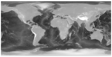
The above step is a local operation whereby each output pixel value is solely influenced by input pixels sharing the same location.
In this step, you will perform another local operation where the output raster will be binary (a value of 0 will represent water pixels and a value of 1 will represent land pixels). The input elevation values will be used to determine the cutoff (i.e. all elevation pixels greater or equal to zero will be 1 in the output and all values less than zero will be 0).
We will implement two different approaches: one will use the Con() function and the other will use a simple algebraic expression.
Method 1
This method makes use of the Con() function.
Open the Raster Calculator geoprocess tool (under Spatial Analyst Tools >> Map Algebra) then type the expression Con( "Elev.img" >= 0, 1, 0). Note the uppercase “C” in Con (the function is case sensitive).

Save the output raster as land_water.img.
The above conditional statement reads “if a pixel from the Elev.img layer has a value greater than or equal to 0 set the output pixel value to 1 if not, set it to 0”.
Method 2
A more succinct approach to creating the land/water raster is to apply a simple algebraic operation, i.e. “Elev” >= 0.
Open the Raster Calculator geoprocess tool (under Spatial Analyst Tools >> Map Algebra) then type the expression "Elev.img" >= 0.

Feel free to overwrite land_water.img from Method 1, or name the output land_water2.img.
The above condition is evaluated for each pixel, if it’s true (i.e. if the pixel value is greater than or equal to 0), the output pixel of the new raster will be assigned a value of 1 (for TRUE), if not, it will be assigned a value of 0 (for FALSE).
Both methods should produce the same output rasters.
If the raster data has values stored as integers, and “if the range of values in the raster is less than 100,000 or if the number of unique values in the raster is fewer than 500” (see ArcGIS reference) a raster attribute table is usually present.
Access the land_water.img attribute table by right-clicking on the layer
in the TOC.
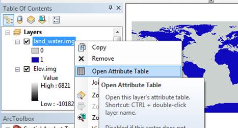
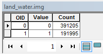
You should see two rows, each indicating the number of times (Count field) a value (Value field) is present in the raster. The value 0 (representing water) is found 391,205 times while the value 1 is found 191,995 times.
Since the pixels (or grid cells) have the same dimensions across the entire
raster extent, the fraction of the earth’s surface covered by water can be
estimated from these pixel counts alone. However, we first need to project the land_water
raster to a coordinate system that preserves area to ensure that
the distribution of land and water pixels are properly represented along the
north-south direction.
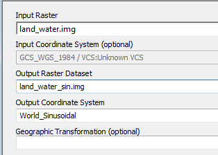
Using the Data Management Tools >> Projections and Transformations >> Raster >> Project Raster tool, project the land_water layer using a world sinusoidal projection (Projected Coordinate Systems >> World >> Sinusoidal (world) ). Name the output land_water_sin.img and make sure to save it in your project folder.
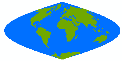
At first glance, the sinusoidal raster does not look different from that of the
unprojected (GCS) raster. However, when zooming in near the polar regions, you’ll
note that the sinusoidal pixels are distorted (i.e. they are not square
shaped).

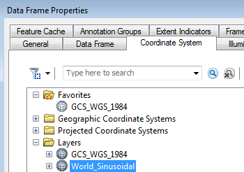
To view the new raster layer in its native coordinate system, change the data frame’s coordinate system to World Sinusoidal by right-clicking on the data frame’s name and selecting Properties then the Coordinate system tab. You can select the coordinate system from the Layer’s folder instead of navigating through the different PCS options.
Note the diminishing number of pixels along the east-west axis when approaching the poles.
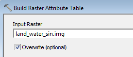
Note: As of version 10.4, ArcGIS may not properly update the count field in the projected raster attribute table. This results in erroneous pixel counts! A workaround is to close the attribute table and run Data Management >> Raster >> Raster Properties >> Build Raster Attribute Table on this table to update the count values.
The new Value counts for 0’s and 1’s should now read 264,984 and 106,082 respectively.
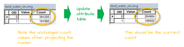
Recall that 0’s represent water, hence the fraction of water covering the earth’s surface can be estimated from this raster as 264,984 / (264,984 + 106,082) = 0.71 (or 71%).
This ends this exercise.
![]() Manuel Gimond, last modified on 7/12/2018
Manuel Gimond, last modified on 7/12/2018