Map Algebra: Zonal and Global Operations
|
1. Create a folder called MapAlgebraZonal somewhere under your personal directory (e.g. C:\Users\jdoe\Documents\Tutorials\MapAlgebraZonal). 2. Download the MapAlgebraZonal.zip data for this exercise and extract the files to your newly created MapAlgebraZonal directory. |
Note that this tutorial will make use of the Spatial Analyst extension, so make sure to enable this extension from the pull-down menu under Customize >> Extensions. Also, all output files should be saved in the current project folder (i.e. ./MapAlgebraZonal).
Step 2: Distance to the closest Walmart
Step 3: Reclassifying raster cells
Step 4: Computing zonal statistics by state
Open the Walmarts.mxd map document.
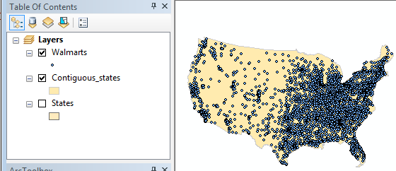
The map consists of Walmart store point locations across the US. This tutorial will explore the use of global and zonal raster operations. The goal will be to explore the average distances to the closest Walmart stores nationwide and within each state. The first step will therefore involve creating a Euclidean distance raster layer from the point layer—a global operation.
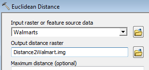
Create a Euclidean distance raster from the Walmart point locations. Use the Euclidean Distance tool found under Spatial Analyst Tools >>Distance Spatial.
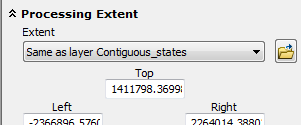
Change the Environment parameters by setting the Processing Extent
to that of the Contiguous_states,
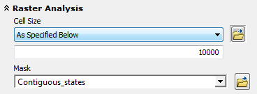
and set the cell size to 10 km (or 10000 meters) and the Raster
Analysis >> Mask to Contiguous_states.
Click OK to close the Environment window and OK again to run the geoprocess.
Note that the mask option will restrict the input points to the extent defined by the mask, this is not a problem here since the mask encompasses all the points. However, if input points are outside of the mask, it’s best to leave the mask field blank and clip the Euclidean distance raster output using the Extract by Mask tool under Spatial analyst >> Extraction.
Note that to view the raster, make sure to turn off any overlaying polygon layers in the TOC.
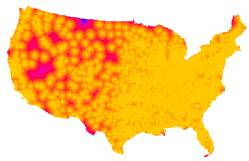
Each pixel of the output raster displays the distance from that pixel to the closest
Walmart. Note that the distance units are those of the map or layer coordinate
system. Also note that the Euclidian distance is sensitive to the coordinate
system used (i.e. you should choose one that preserves distance before
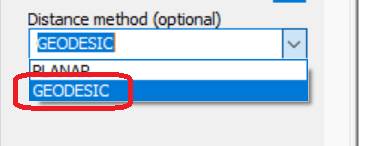
computing the distances). If you are using version 10.7 or greater of the
software, you also have the option of adopting the geodesic method of
distance measurement over the default planar method.
Next, you will identify all pixels that are within 20 km of a Walmart.
Reclassify the Euclidean distance raster to binary values: 0’s for distances greater than 20 km and 1’s for distances less than or equal to 20 km. There are at least two ways in which this step can be accomplished: one approach is to use the Raster Calculator tool and the other is to use the Reclassify tool. Regardless which method you choose to use make sure to name the output raster Dist20k.img.
Method 1: Raster Calculator
Open Spatial Analyst Tools >> Map Algebra >> Raster Calculator.
In the expression box, type Con( "Distance2Walmart" <= 20000, 1, 0)
![]()
Click OK to run the geoprocess.
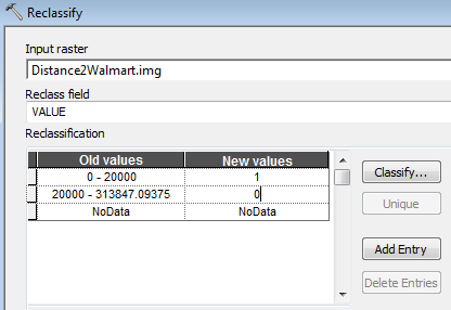
Method 2: Reclassify
Open Spatial Analyst Tools >> Reclass >> Reclassify.
Populate the fields as shown
below (you may need to delete rows in the reclassification table or you can
define the classification limits via the ![]() button).
button).
Click OK to run the
reclassification
The output map will be a binary raster.
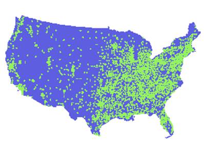
As such it will have a valid attribute table listing the number of 0 and 1 pixels in the raster.
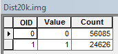
From these values we can compute the percentage of all locations within the 48 states that are within 20 km of a nearest Walmart, or 24626 / (56085 + 24626) = 30.5%.
In the next step, you will learn how to summarize pixel values by state using a zonal operation.
Open the Zonal Statistics as Table tool (Spatial Analyst Tools >> Zonal >> Zonal Statistics as Table). The zone layer can be either a raster or a vector. In this working example, we will use the States vector layer as the zonal boundaries.
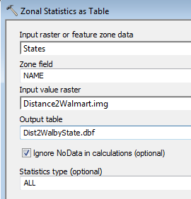
Click OK to run the geoprocess.
Note that the output is a simple table (in a dbf file format) and not a spatial data layer. You can view its contents by right-clicking it in the TOC then selecting Open.
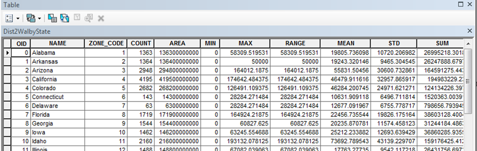
For each polygon in the States layer, a set of distance-to-Walmart summary statistics is tabulated. The output table copies the NAME column from the input States layer—this will allow us to join this table back to the States vector layer.
Right-click on the States layer in the TOC then select Joins and Relates >> Join.
Populate the fields as follows:
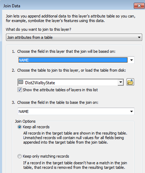
Click OK to perform the join. (If you are prompted to create an index, click Yes).
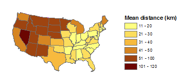
The States layer can now be symbolized using data from the summary statistics table. In the following example, the layer is symbolized by the mean distance to the nearest Walmart.
Note: This exercise uses polygons as input feature zones in the Zonal Statistics as Table tool however, note that you can also use point features as input feature zones.
![]() Manuel Gimond, last
modified on 10/16/2019
Manuel Gimond, last
modified on 10/16/2019