Quantifying Point Patterns
|
· Create a folder called PPA somewhere under your personal directory (e.g. C:\Users\jdoe\Documents\Tutorials\PPA). · Download the PPA.zip data for this exercise and extract the files to your newly created PPA directory. |
This tutorial makes use of a tropical forest census which plots the positions of 3605 trees of the species Beilschmiedia pendula (Lauraceae) in a 1000 by 500 meter rectangular sampling region in the tropical rainforest of Barro Colorado Island. This version of the data was pulled from the spatstat R package.
Source: Condit, R. (1998) Tropical Forest Census Plots. Springer-Verlag, Berlin and R.G. Landes Company, Georgetown, Texas.
Parts of this tutorial requires that you enable the Spatial Analyst extension under Customize >> Extensions.
Step 1: Density based: Gridded quadrat count
Step 2: Density based: Tessellated quadrat count
Step 3: Density based: Point density tool
Step 4: Density based: Kernel density tool
Step 5: Distance Based: nearest neighbor tool
Open the Point Pattern.mxd document.
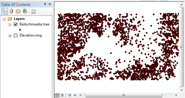
The map consists of a layer, Beilschmiedia tree, that plots the location of 3605 trees. It is assumed to be a complete census of trees. The Elevation.img layer is a raster of elevation values recorded in meters.
First, we’ll create a uniform grid (5 rows by 10 columns) using the Data Management >> Sampling >> Create Fishnet tool from ArcToolBox. Make sure to set the grid extent such that the x-axis covers a range of 0 to 1000 (meters) and the y-axis covers a range of 0 to 500 (meters). Set the output type to Polygon and name it Grid.shp.
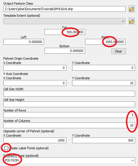
Click OK to run the geoprocess.
Note that the map’s coordinate system is not explicitly defined, but as long as we know that the trees were recorded in a local Cartesian coordinate system that preserves distance, we should be fine.
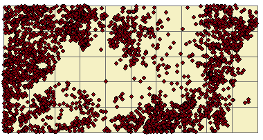
Next, we will tally the number of trees within each grid cell.
Right-click on the newly create Grid layer and select Joins and Relates >> Join. In previous tutorials we’ve used this tool to join tables, here, we’ll use the spatial join option instead.
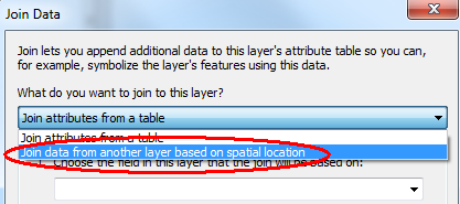
The layer whose features will be tallied in the Grid layer is the Beilschmiedia tree layer. By default, this tool will compute the total number of points in each grid cell so we do not need to compute any other summary. We’ll name the output Join_Output.shp.
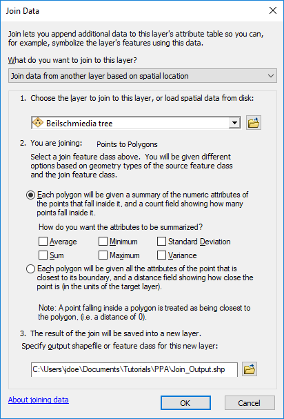
Click OK.
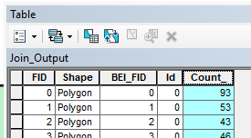
The output shapefile has a field called Count_ that tallies the points in each polygon.
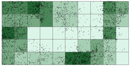
Change Join_Output’s symbology to reflect the Count_ values.
Step 2: Density based: Tessellated quadrat count
In the last step, you created quadrats from a uniform grid. Quadrats need not be uniform in shape and in size. In this step, you will create quadrats based on elevation intervals for the purpose of counting the number of trees at different elevation ranges.
We’ll first reclassify the raster into four
elevation intervals (each classification bin covering an equal range) using Spatial
Analyst Tools >> Reclass >> Reclassify. We will create equal
interval classes so make sure to select the Equal Interval method from
the Classification window (accessed via the ![]() link). You will
probably want to bump the upper range value to 160 to ensure that all
input values are reclassified.
link). You will
probably want to bump the upper range value to 160 to ensure that all
input values are reclassified.
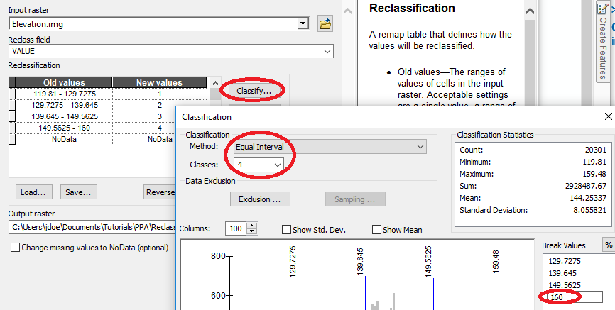
Before running the Reclassify tool, we might want to set the lower bound to a smaller value like 119, to make sure that we are not excluding values due to rounding errors. This can be done directly in the reclassification table.
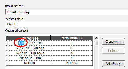
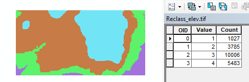
Name the output Reclass_elev.tif then click OK to run the geoprocess.
Next, we’ll convert the categorical raster to a vector layer. Note that this new raster has an attributes table whereas the original raster did not. This is to be expected since the newly created raster has just 4 unique integer values (ArcMap will not create a raster attributes table if there are too many unique pixel values).
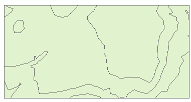
In ArcToolbox, select Conversion Tools >> From Raster >> Raster to Polygon and populate the fields as follows:

The output is a polygon vector layer.
Next, we’ll tally the number of points in each tessellated surface using the spatial join workflow described earlier.
Right-click the quadrat_tess layer and select Joins and Relates >> Join. Populate the fields as follows:
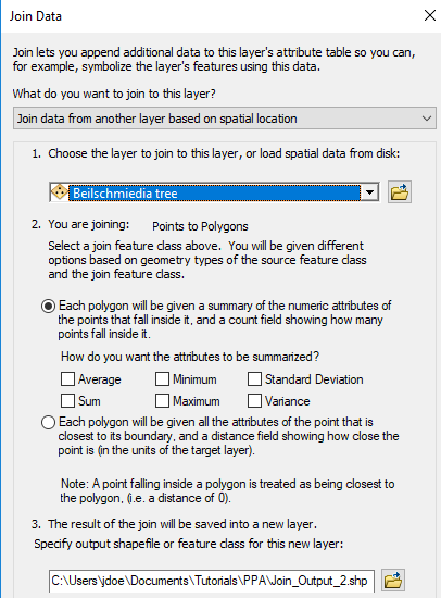
Click OK to perform the spatial join.
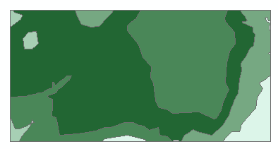
Symbolize the newly created Join_Output_2 layer using the Count_ field.
If you look at the attributes table, you’ll note the one-to-one relationship between polygons and attribute values.
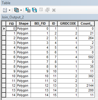
We will want to reduce the number of records to just four (one for each unique elevation interval) using the dissolve tool. Note that the elevation interval value is named GRIDCODE (this is the default vector attribute name when converting from raster to vector).
From the Geoprocessing pull-down menu select Dissolve. Set Join_Output_2 as the input layer. Select gridcode as the dissolve field. From the Statistics Fields(s) pull-down menu select Count_. This attribute will be added to the Field list below. Then select SUM as the statistic type. Name the output Join_Output_2_dis.shp.
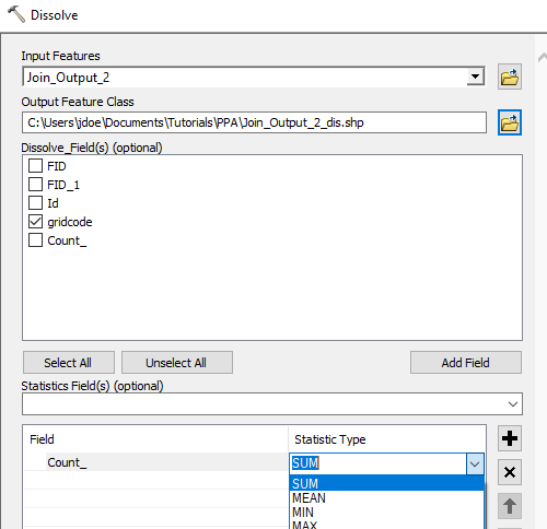
Click OK to dissolve the layer.
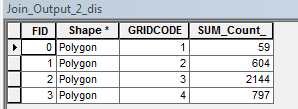
The new shapefile now has just four records (a one-to-many relationship).
We could compare the counts between all four elevation intervals however, the area of each interval may not be the same (recall the modifiable aerial unit problem). So we should normalize the count to area. This will require that we create two new attribute fields: Area and Density (both data types stored as Float).
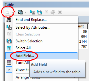
Add two new fields from Add Field option: Area and Density. Make sure to set their types to Float.
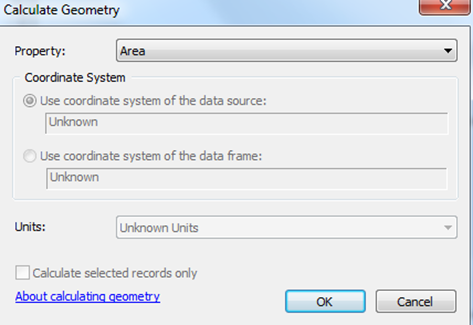
For the Area field, compute its area by right-clicking the column header >> Calculate Geometry.
Click OK to compute the area.
Note that the coordinate system is in meters (even though it’s not explicitly defined in the layer’s CS).
For the Density field, type in the expression [SUM_Count_]/[Area] via right-clicking the column header >> Field Calculator:
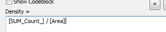
Click OK to compute the values.
The attributes table should look like this:
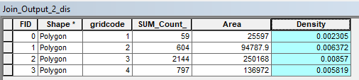
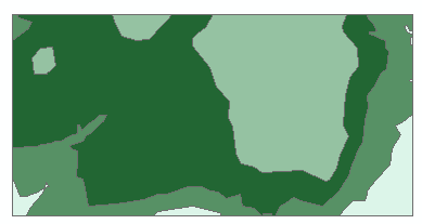
Symbolize join_Output_2_dis using the Density Attribute.
Finally, we can make use of ArcGIS’ rudimentary chart tool to plot count vs elevation range.
From the View pull-down menu select Graphs >> Create Graphs and populate the fields as follows:
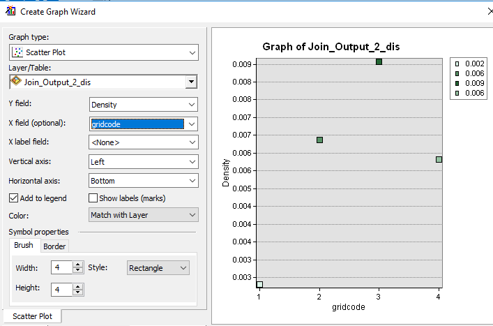
The plot suggests a peak tree density at the third elevation interval (elevation of 139.6 m to 149.6 m, roughly). Note that the point symbol colors match those of the input shapefile. This facilitates matching plot points to map polygons.
You can save the plot or dismiss it.
In this step we’re creating a density map of tree counts.
In ArcToolbox open Spatial Analyst Tools >> Density >> Point Density.
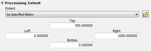
Since the geoprocess will create a new raster from a vector layer, it may not be a bad idea to explicitly define the raster extent since the tool will default to the smallest rectangle encompassing the input point layer.
Open the Environments setting and define the extent as outlined below:
Click OK to close the Environments setting and populate the Point Density tool fields as follows:
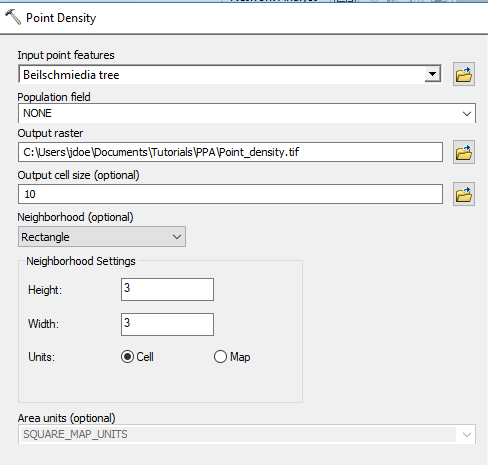
Click OK to run the geoprocess.
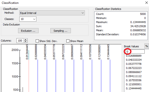
Set the new raster’s symbology classification scheme to equal interval (10 classes) via its Properties >> Symbology menu. Ensure that the lower value is set to 0.
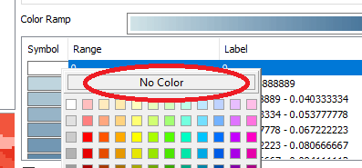
Assign No Color to the pixel value of 0.
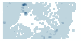
Your output should look something like this.
Each pixel is assigned the number of points within a 3x3 pixel search window then divided by the area of that search window. For example, if a cell has one point inside the search window, its output value will be:
1 point / (9 cells * 100m2 area per cell) = 0.0011 points per square meter (within a 3x3 search window)
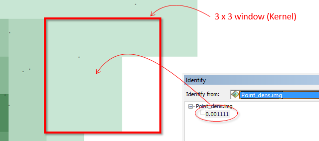
Note that the point density function is a focal operation; behind the scenes, ArcMap converts the point layer to a raster before computing the output density values.
ArcMap offers two density tools: a point density (covered in the last step) and a kernel density tool. This would seem to suggest that these tools perform distinct operations when in fact the point density tool is simply a special case of a kernel density function whereby all input values in the focal operation are assigned equal weight. ArcMap’s Kernel density tool applies a quartic function that assigns a non-uniform weight to each point based on its proximity to the output cell. This tool tends to generate smoother density rasters.
In ArcToolbox open Spatial Analyst Tools >> Density >> Kernel Density. Set the extent in the Environments window as outlined in the previous step then populate the fields as follows:
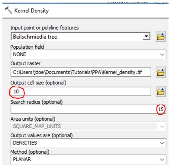
Note that this tool only allows you to define a kernel by its search radius and not by cell grids. Here, we use a 15 m search radius.
Click OK to run the geoprocess.
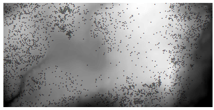
Next, generate a symbology scheme similar to the one used in the last step (make sure to set 0 pixel values to no color).
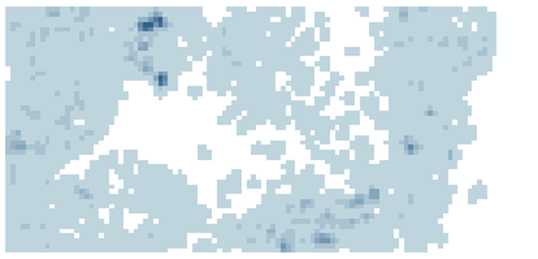
Note the smoother appearance of density values compared to
the Point Density tool output.
Step 5: Distance Based: nearest neighbor tool
So far, we’ve explored density based approaches to quantifying point patterns. Density based analysis usually focuses on a point pattern’s first order property—i.e. its distribution vis-à-vis location. Another property of interest is a point pattern’s spatial interaction, a second order effect. A statistic that can be used to quantify a point pattern’s second order property is the average nearest neighbor (ANN) statistic.
In ArcToolbox, open Spatial Statistics Tools >> Analyzing Patterns >> Average Nearest Neighbor and populate the fields as follows (make sure to check the Generate Report option).
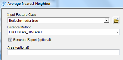
Click OK to run the tool.
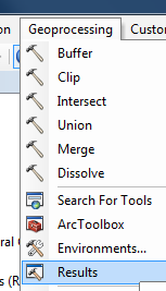
The output is not a data layer but a report saved as an HTML file. To view this file, open the Results tab from the Geoprocessing pull-down menu.
In the Results tab, expand Current Session >> Average Nearest Neighbor (if you ran more than one ANN analysis, pick the top-most instance).
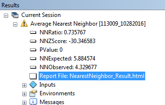
You might notice a yellow warning symbol next to the geoprocess. It’s simply indicating that the tool does not recognize this layer as being in a projected (Cartesian) coordinate system. Recall that the file has no defined CS, but it is assumed that the tree locations were geo-located on a planar coordinate system. This is a good reminder that this tool measures planar distances and not geodesic distances.
Double-click on the Report File:NearestNeighbor_Result link.
You will ignore the infographic at the top of the report (this tutorial does not cover hypothesis testing) and focus on the first row of the summary table which gives us the average distance between all nearest neighbor combinations.
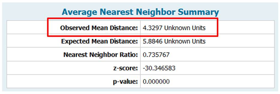
The coordinate system was never explicitly defined in this layer so the software defines the units as “unknown”. This is fine since we know that the units are in meters. The output indicates that the average distance between first order neighboring trees is about 4.3 meters.
The study area was not explicitly defined in this step (last input field of the ANN tool). This does not influence the observed mean distance measurement. However, if you are to make use of any of the other output elements, you should explicitly define the study area since this value is used to compute the other output elements such as the expected mean distance value.
![]() Manuel Gimond, last modified on 10/26/2018
Manuel Gimond, last modified on 10/26/2018