Tissot’s Indicatrix Circles
|
1. Create a folder called Tissot somewhere under your personal directory (e.g. C:\Users\jdoe\Documents\Tutorials\Tissot). 2. Download the data for this then extract the files from the Tissot.zip file to your newly created Tissot directory. |
|
In the nineteenth century, Nicolas Auguste Tissot developed a
method to analyze map projection distortion. [src: ESRI] |
|
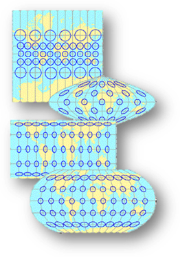
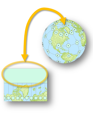
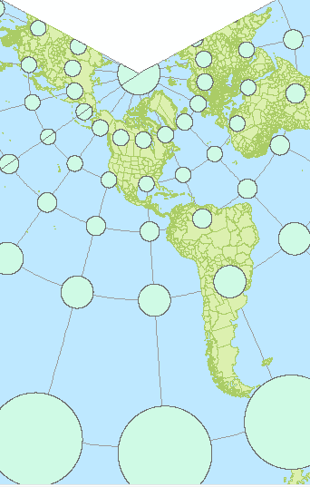
In this exercise, you will create geodesic circles on a spheroid representation of the earth. These circles will be used as a reference to evaluate the distortion in shape and area that accompany most projected coordinate systems. You will be introduced to the following tools and concepts:
· using the buffer tool to create geodesic circles,
· changing a data frame’s coordinate system,
· modifying a coordinate system’s parameters,
· measuring a feature’s surface area and dimensions using the measurement tool,
· ArcGlobe.
Step 3: View the Tissot circles in ArcGlobe
Step 4: View Tissot’s circles in a modified orthogonal projection
Step 5: View Tissot’s circles in other projections
Step 6: Explore other projections on your own
Navigate to your Tissot project folder and double click Tissot.mxd. This should launch Arcmap.
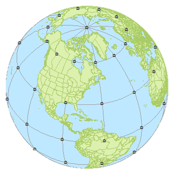
The map is composed of a political boundaries layer, a graticule layer and a 30° x 30° grid of points. ArcMap allows you to work with layers having different coordinate systems within the same map document. All layer coordinate systems are re-projected to that defined by the data frame. In this example the data frame’s coordinate system is set to an orthographic projection (as seen from space). However, the data are all in a geographic coordinate system (i.e. they are unprojected).
An easy way to create a circle (planar or geodesic) from points is to use the buffer geoprocessing tool.
If ArcToolbox is not open, open it by clicking on ![]() .
.
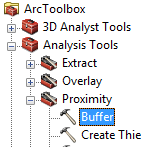
In ArcToolbox, open Analysis Tools >> Proximity >> Buffer. (Note that the same Buffer tool can also be accessed from the Geoprocessing pull-down menu).
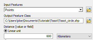
In the Buffer window, select the Points layer as the Input feature, name the output Tissot_circle.shp and specify 600 kilometers for the liner unit (this is the buffer’s radius value).
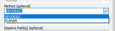
Buffer creation is sensitive to coordinate systems used. So if you want to create a perfect circle that covers a relatively large region while avoiding distortions that can accompany some projected coordinate systems, it’s best to create a geodesic buffer output. A geodesic feature is one that is created on a sphere or ellipsoid and not on a plane.
Note that the geodesic option in the buffer tool is only available in ArcMap 10.4.1 or later. If you have an older version of ArcMap, a solution is to set the output coordinate system in the Buffer tools environment settings to a geographic coordinate system such as WGS 1984.
Select GEODESIC from the Method pull-down menu.
Click OK to start the Buffering process.
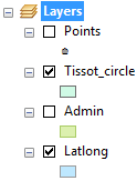
Once the buffer process is complete, a new layer called Tissot_circle will be added to your map.
Save the map document by clicking on the Save
button ![]() .
.
Next, we take a closer look at the Tissot circles on a 3D globe
On your Windows desktop, click on the Windows ![]() icon
and open ArcGIS >> ArcGlobe 10.x.
icon
and open ArcGIS >> ArcGlobe 10.x.
ArcGlobe is similar to Google Earth. It allows you to display ArcGIS layers on a 3D globe.
If an ArcGlobe - Getting Started window pops up, click OK to accept the default settings.
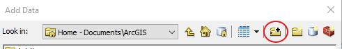
Click the Add Data button ![]() .
.
You might need to create a folder connection to your Tissot workspace.
In the Add Data window, click on the Connect to Folder button.
In the Connect to Folder window, navigate to your Tissot folder and select it.
In the Add Data window, navigate to your Tissot project folder and select Tissot_circle.shp.
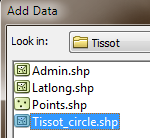
Click Add to close the Add Data window and load the Tissot_circle layer.
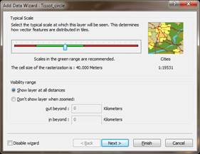
If an Add Data Wizard window pops up click Finish to accept all default settings.
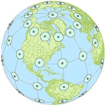
At this point, you will see the earth globe but you may not see the circles. This is because the Tissot_circle layer is hidden behind the Imagery layer (remember that layers are drawn in the order listed in the TOC from bottom to top).
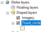
In the TOC, drag the Tissot_circle layer above the Imagery layer.
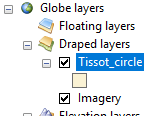
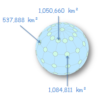
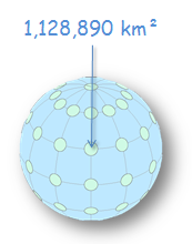
The circles should now appear. Rotate the globe with the cursor. You should see little distortion in the circles.
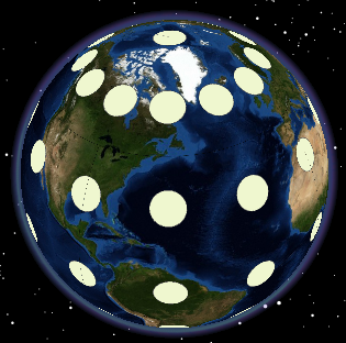
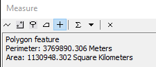
Next we will check the circle’s surface area. If true surface area is preserved, the area of each circle feature should approximate pr² or 3.14 x 600² = 1,130,973 km².
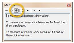
In ArcGlobe, click on the Measure tool ![]() .
.
Select the Measure a Feature tool.

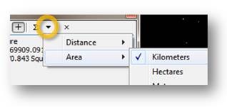
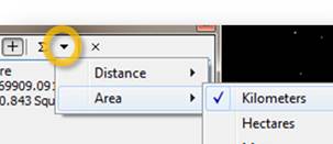
Change the area units to square kilometers by clicking on the “inverted” triangle and selecting Area >> Kilometers.
With the measure tool active, click on any circle except those at each pole (the polar circles are not perfect circles since they are generated across a boundary extent).
The values returned should be very close to the theoretical value of 1,130,973 km².
Now that we’ve confirmed that the circles generated in Step 1 are close-to-perfect geodesic circles, we can move on to the next step.
Close ArcGlobe. You do not need to save the ArcGlobe project.
Navigate back to your ArcMap Tissot.mxd project (if you closed the ArcMap window in a previous step, re-open it).
To speed up the drawing time, turn off the Points and Admin layer for now.
You will now study the circles’ shapes and sizes in different projections.
In the TOC, right-click on the Layers data frame and select Properties.
In the Data Frame Properties window, select the Coordinate System tab.
Note that the Data frame’s current coordinate system is The_World_From_Space which is an Orthographic projected coordinate system.

This projection is used to visualize the earth as it would be seen from space. But, as you will learn in the following steps, even though the circles are displayed as they would be seen from space, Arcmap does not see the displayed circles from a 3D perspective but from a planar perspective instead.
Close the Data Frame Properties window by clicking OK.
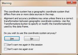
If you get the following warning window, click Yes to close it.
Click on the Measure tool ![]() .
.
Select the Measure a Feature tool.
Change the area units to square kilometers if the area value is in a different unit by clicking on the “inverted” triangle and selecting Area >> Kilometers.
With the measure tool active, click on any circle other than the ones at each pole.
You’ll probably note that each circle area is different. ArcMap is interpreting the shape of the circles as they are displayed in the View window (i.e. the features are now interpreted as different sized ellipses).
However, the closer the circle feature is to the center of the view extent, the closer its area value is to the theoretical area value. This is the nature of an orthographic (planar) projection. Features closest to the center of the map extent (i.e. the location where the projected plane touches the earth surface) suffer less distortion in area, shape and orientation than those further away.

You can modify the location where the projected plane touches the earth surface in the coordinate system properties window.
In the TOC, right-click on Layers data frame and select Properties.
In the Data Frame Properties window, select the Coordinate System tab.
Right-click the The World from Space and select Copy and Modify.
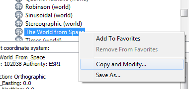
In the Projected Coordinate System Properties window, change the Longitude_Of_Center value to -60.0 and the Latitude_Of_Center value to 30.0.
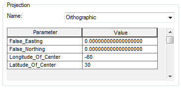
The above coordinates should place the center of the map extent at one of the Tissot circles.
Click OK to close the Projected Coordinate System Properties window.
Click OK to close the Data Frame Properties window.
If you get a warning window, click Yes to close it.
Click on the Measure tool ![]() .
.
With the measure tool active click on the circle closest to the extent center.
The areal value should be around 1,128,870 km². This is not quite the theoretical value of 1,130,973 km² we were expecting. The reason is that distortion increases as soon as you move away from the projection center (which is at 60°W and 30°N in our example). Since the circle features are polygons and not points, distortion will increase as their sizes increase.
Now, we will explore other popular projections and observe the varying forms of distortions one should anticipate when using those projections.
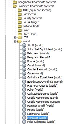
The first projection we’ll explore is the popular Mercator projection (a cylindrical projection).
In the TOC, right-click on the Layers dataframe and select Properties.
Change the data fame’s CS to Projected Coordinate Systems >> World >> Mercator (world).
Click OK to close the Data Frame Properties window.
Turn on the Admin layer in the TOC for
background reference. You might need to zoom to the map’s full extent ![]() .
.
Note the different sized circles. Remember that these are the original circles of equal area and shape. This Mercator projection distorts area but preserves shape. Using the measure tool, you’ll find that the circles vary from 4,568,587 km² at 60°N to 1,132,631 km² near the equator. The Mercator projection does a much better job preserving all features’ geometric attributes near the equator.
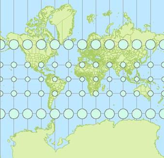
You may have also noticed bands similar in color to the Tissot circle’s at the top and bottom of the map extent. These are the polar indicatrices. Note their distortion!
Let’s explore another projection: Cylindrical Equal Area.
In the TOC, right-click on the Layers data frame and select Properties.
Select Projected Coordinate Systems >> World >> Cylindrical Equal Area (world).
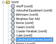
Click OK to accept the changes.
Like the Mercator projection, this is a cylindrical projection. However, instead of preserving shape like the Mercator projection, this one preserves area. Using the measure tool, you’ll find that the circles vary from 1,130,117 km² at 60°N to 1,130,109 km² near the equator. The values are less than 0.001% off from the theoretical value. Not bad!
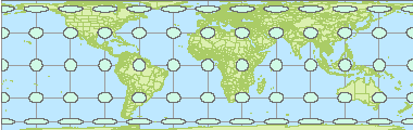
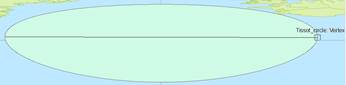
However, along with a relatively accurate surface area representation comes some serious distortion in shape.
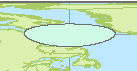
Zoom-in on one of the circles along the 60° line of latitude.
Click on the Measure tool ![]() .
.
In the Measure tool window, click on the Measure Line
button ![]() .
.
In the View window, move the cursor near the top of the distorted circle until it ‘snaps’ near the top most vertex. Start the beginning of the line measurement by left-clicking at the snap location.
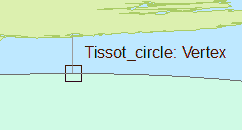
Next, move the cursor near the bottom of the circle until you feel it “snap” near the bottom most pixel. Once snapped, double-click on that point to end the line measurement segment.
The distance between the top most and bottom most vertices should be around 600 km. This makes sense since the cosine of 60° is 0.5 or half of the circle’s diameter, 1200/2 = 600 (distortion in this projection is proportional to the cosine of the latitude).
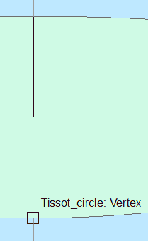
Now measure the distance between the left most and right most vertices of the distorted circle.
The distance between the left most and right most vertices should be somewhere around 2400 km.
If area is a spatial property that you want to preserve, a cylindrical equal-area projection is a good coordinate system candidate.
Let’s explore a continent based projected coordinate system.
In the TOC, right-click on the Layers data frame and select Properties.
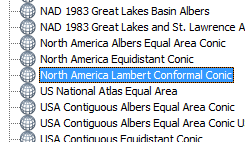
Select Projected Coordinate Systems >> Continental >> North America >> North America Lambert Conformal Conic
Click OK to close the Data Frame Properties window.
If a warning message window pops up, click Yes.
This projected coordinate system is a conical coordinate system. It is also a conformal coordinate system which preserves shape. Note how all of the circles remain perfect circles. But, as you probably noticed by now, the circle’s area is not preserved. However, the surface areas remain consistent along the lines of latitude. In our example, the surface area for the circles range from 37,038,000 km² (at 60°S) to 1,035,000 km² (at 30°N). For North America, the surface area measurement error can be as great as 8%.
Let’s look at a more localized projected coordinate system.
In the TOC, right-click on Layers and select Properties.
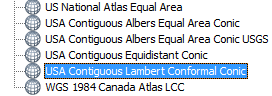
Select Projected Coordinate Systems >> Continental >> North America >> USA Contiguous Lambert Conformal Conic.
Click OK to close the Data Frame Properties window.
If a warning message window pops up, click Yes.
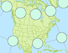
This conical projected coordinate system does a better job in preserving area for the US and southern Canada. In our example, the surface area for the circles in our region range from 1,147,000 km² (at 30°N) to 1,308,000 km² (at 60°N). The area measurement error for the 48 states falls well within 2%.
Feel free to explore the properties of other projected coordinate systems and note the type of distortions they present.
![]() Manuel Gimond, last modified on 7/11/2018
Manuel Gimond, last modified on 7/11/2018