Creating a Human Influence Index map
|
1. Create a folder called HII somewhere under your personal directory (e.g. C:\Users\jdoe\Documents\Tutorials\HII). 2. Download the data for this exercise then extract the files from the HII.zip file to your newly created HII directory. This exercise requires the use of the Spatial Analyst extension. The extension can be activated under Customize >> Extensions. |
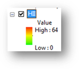
In this exercise, you will create a Human Influence Index (HII) map for the state of Maine following the methodology outlined by E.W. Sanderson (http://sedac.ciesin.columbia.edu/wildareas/methods.jsp). The HII values range from 0 (no human influence) to 64 (maximum human influence). Different data layers have different influences on the HII score as shown in the following table:
|
Variable category |
Influence Score |
|
Influence of Population Density/km² 0 - 0.5 |
0 |
|
Influence Score of Railroads Within 2 km of
railroads |
8 |
|
Influence Score of Major Roads Within 2 km of roads |
8 |
|
Influence Score of Navigable Rivers Within 15 km of
navigable rivers |
4 |
|
Influence Score of Coastlines Within 15 km of
coastlines |
4 |
|
Influence Score of Nighttime Stable Lights Values 0 |
|
|
Urban Polygons Inside urban polygons |
10 |
|
Land Cover Categories Urban areas |
10 |
Since HII values need to be computed for all locations across the state of Maine, the HII layer needs to be a continuous raster data layer. You will use different geoprocessing tools to derive the HII raster layer. Stepping through each geoprocess (more than a dozen) can be time consuming, especially if the process needs to be repeated several times. ArcGIS has a modeling option that allows the user to connect many geoprocesses needed to complete a task. This has the benefit of allowing one to (1) rerun the model with different datasets or parameters more quickly and following a systematic process and (2) test the model using small data sets before running the model on larger ones that can take hours or days to complete.
In this exercise you will learn to:
· convert vector data to raster data,
· create Euclidean distance raster,
· reclassify raster values,
· sum raster layers,
· create a geoprocess model.
Step 2: Converting vector layers to raster layers
Step 3: Automate geoprocessing with ModelBuilder
Step 4: Setting model parameters
Step 5: Adding a Euclidean Distance tool to the model
Step 6: Adding a reclassification tool to the model
Step 7: Adding a Raster Calculator tool to the model
Launch ArcGIS from Start >> All Programs >> ArcGIS >> ArcMap.
Select Existing Maps >> Browse for more.
![]()
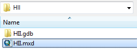
Navigate to the HII and select HII.mxd.
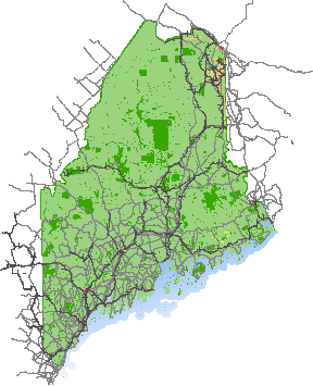
In the right window pane (referred to as the Data View window), you see a map of the state of Maine with various data layers showing roads, railways, urban areas, etc...
In the left-side window pane (referred to as the Table of
Content or TOC for short), you see a list of data layers that can be turned on
and off. Some are already turned on while others are not. Turn each layer on
and off to familiarize yourself with the datasets you will be working with. Use
the zoom tools ![]() and the pan tool
and the pan tool ![]() to explore the data
at different scales.
to explore the data
at different scales.
There are two vector layers that need to be converted to rasters for the analysis: pop_dens (population density layer) and urban (polygon layer that identifies urban areas).
If not already opened, open the Toolbox by clicking on
the Toolbox button ![]() .
.
You will use one of ArcGIS's extensions: Spatial Analyst. This extension needs to be activated.
From the Customize pull-down menu select Extensions.
Turn on the Spatial Analyst extension by checking the box next to the extension.
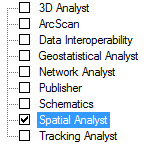
Click Close to close the Extensions window.
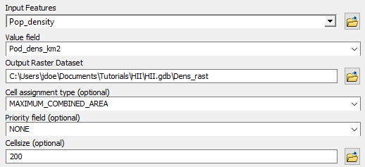
You will convert the population density layer to a raster layer. The new raster layer will be computed using Pop_density's population density (Pod_dens_km2) attribute.
In ArcToolbox, expand Conversion tools. Then expand the To Raster toolset.
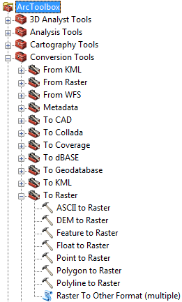
Double-click Polygon to Raster ![]() .
.
Fill in the fields as shown in the following graphic.
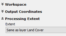
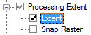
Click on the Environments button (located near the bottom of the Polygon to raster tool) to access additional settings.
Expand Processing Extent.
Change the Extent to Land Cover.
Scroll down the Environment Settings window and expand Raster Analysis.
Set the Mask to Land Cover.
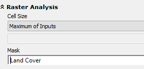
A mask clips the output raster to an existing layer (Land Cover in this exercise).
Click OK to close the Environment Settings window.
Click OK to start the polygon-to-raster conversion geoprocess.
The geoprocess status bar will appear at the bottom of the window. Note: When you first run a geoprocess, it may take several seconds before the status bar appears.
![]()
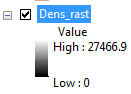
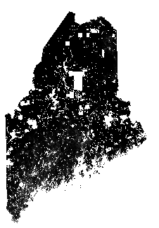
When the process is complete, the status bar will disappear. You should now see a new raster layer called Dens_rast added to your map document.
In the TOC, turn all layers off except Dens_rast by unchecking the checkboxes next to the layers that are checked.
Your Data View should now only display the newly created Dens_rast layer.
You will change the raster layer's symbology to improve the visual distinction between areas of high and low population density.
In the TOC, double-click the Dens_rast layer to access its properties.
Click on the Symbology tab ![]() .
.
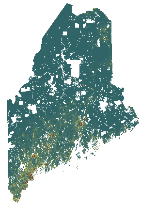
Change the color ramp to a red-green color scheme.
Check the Invert box to invert the color scheme so that red is associated with high numbers and green is associated with low numbers.
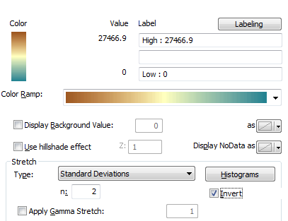
Your map should now effectively show areas of high population density.
In the TOC, turn on the Urban layer ![]() .
.
The Urban layer is represented using non-contiguous polygons. You will need to zoom in on densely populated areas (e.g. Portland, Bangor, etc..) to see the polygons. You might need to toggle the Dens_rast layer on and off to identify the Urban polygons in the map.
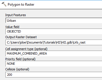
Next, you will perform the same Polygon-to-Raster conversion on the Urban polygon layer.
In ArcToolbox, open Conversion >> To Raster >> Polygon to Raster.
You will populate the fields as follows:
Click on the Environments button.
Change the environment settings like you did for the Polygon-to-Raster conversion performed with the Pop_density layer (i.e. Processing Extent >> Extent set to Land Cover and Raster Analysis >> Mask set to Land Cover).
Click OK to accept the Environment Settings changes.
Click OK to start the polygon-to-raster conversion process.
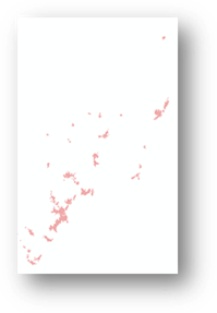
The Urb_rast layer is displayed as a continuous raster layers, however, the non-null values associated with each pixel (i.e. all pixels with a numeric value) are meaningless in this case. That’s because we assigned the shapefile’s OBJECTID value to each pixel. The OBJECTID is nothing more than an identification tag—it does not provide any meaningful information. The Urb_rast layer does nothing more than locate the urban areas within the state of Maine (i.e. presence or absence of urban centers). We will therefore assign the same color to all pixels.
In the TOC, right-click on Urb_rast and select Properties.
Under the Symbology tab, select Unique Values.

In the symbols window select the first symbol under <Heading>.

Scroll down the symbols list until you see the last symbol.
While pressing and holding the Shift key, select the last symbol (symbol 30) in the symbols list.
Pressing and holding he Shift key allows you to select a large range of values.
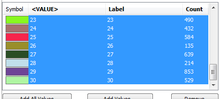
Click on the Remove button ![]() .
.
You should now be left with a single symbol <all other values> in the symbols list.
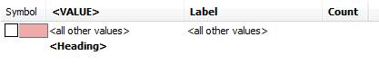
Check the box next to the symbol ![]() .
.
Click OK to accept the changes.
All Urb_rast pixels are now assigned the same color.
There will be many more geoprocessing steps that will need to be completed. This can be time consuming and also prone to input errors. We can create a geoprocess model that will help alleviate some of the aforementioned problems.
First, we will need to create a new Toolbox. We will create one in ArcCatalog.
From the Windows pull-down menu select Catalog.
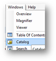
The Catalog window will pop-up on the right side of the ArcMap window. If it collapses back to the right margin, just click on the Catalog tab to access its contents.
To prevent the Catalog window from collapsing back into
the margin, click on the Auto-hide pin ![]() in
the upper-right corner of the Catalog window.
in
the upper-right corner of the Catalog window.
Once “pinned”, the Auto-Hide icon should look like ![]() .
.
In the Catalog window, navigate to the HII geodatabase.
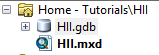
Right-click on HII.gdb and select New >> Toolbox.
The Toolbox can contain more than one geoprocess model. For this exercise, you will create one model in the new toolbox.
Right-click on the newly created toolbox and select New >> Toolset.
Right-click on the newly created Toolset and select Rename.
Rename the Toolset HII.
Right-click on the HII toolset and select New >> Model.
A new Model window should pop-up. This is where you will define the different geoprocessing steps.
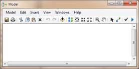
You will change the model parameters that will apply to all geoprocesses in the model.
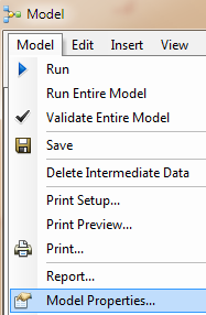
From the Model pull-down menu in the Model window, select Model Properties.
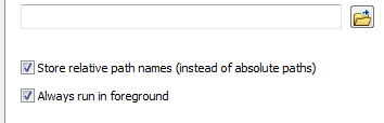
Check the box next to Store relative path names (instead of absolute paths).
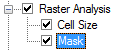
In the Model Properties window, select the Environments tab.
Expend Procession Extent and place a check mark next to Extent.
Expend Raster Analysis and place a check mark next to Cell Size and Mask.
Next, you will set the values for the parameters you just checked off.
In the Model Properties window, click on the Values
button ![]() .
.
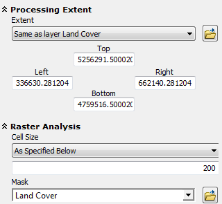
In the Environment Settings window set the parameters values as follows:
· Processing Extent >> Extent: Same as layer Land Cover (the coordinate values will be automatically populated)
· Raster Analysis >> Cell size: As Specified below >> 200
· Raster Analysis >> Mask: Land Cover
Click OK to close the Environment Settings window.
Click OK to close the Model Properties window.
Make a habit of saving your model on a regular basis.
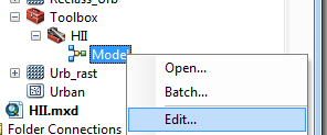
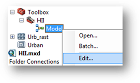
If you need to close the model and return to it at a later time, you can access it by right-clicking on the model in your custom Toolbox and selecting Edit. DO NOT double-click it as this will bring up a blank menu window.
You can add geoprocesses to the model by dragging and dropping tools from the Toolbox to the model.
In ArcToolbox, expand the Spatial Analyst Tools toolbox.
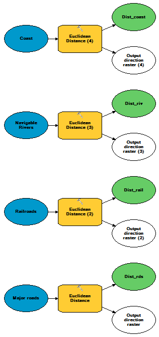
The HII is dependent on the proximity to different anthropogenic and natural features (see HII scores table in the introduction). We therefore need to create GIS layers that will provide us with distances from any location within the state of Maine to any feature of interest (i.e. roads, railways, waterways, etc…). You will use ArcGIS’ Euclidean Distance tool to create these rasters.
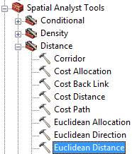
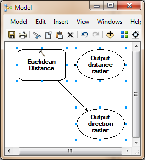
In ArcToolbox, expand the Distance toolset (in the Spatial Analyst Tools toolbox) and drag-and-drop the Euclidean Distance tool into your HII model.
A new (empty) Euclidean Distance tool should now be displayed in your HII model
Next, you will set the input/output parameters for the Euclidean Distance tool.
Double-click the Euclidean Distance tool that you just added to your HII model.
Define the input/output parameters as follows:
· Input raster of feature source data: Major roads
· Output distance raster: …\HII\HII.gdb\Dist_rds
· Output cell size: 200 (this value should already be set by the environments setting)
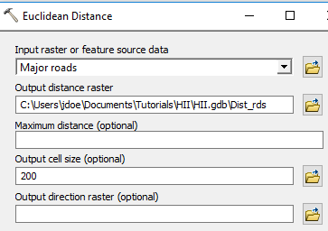
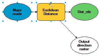
Click OK to accept the changes.
You will probably note that the tool “bubbles” changed color. This indicates that tool paramaters have been set.
You will create three more Euclidean Distance processes in your model for railroads, navigable rivers and coastline.
Drag and drop the Euclidean Distance tool inside your HII model three more times.
For each Euclidean tool, set the parameters as follows:
|
Euclidean Distance process |
Input layer |
Output layer |
Output cell size |
|
Distance to nearest railroad |
Railroads |
.\HII.gdb\Dist_rail |
200 |
|
Distance to nearest navigable waters |
Navigable rivers |
.\HII.gdb\Dist_riv |
200 |
|
Distance to nearest coatline |
Coast |
.\HII.gdb\Dist_coast |
200 |
You can have ArcMap automatically rearrange the tools for
you inside the ModelBuilder by clicking on the Auto Layout ![]() button. You can then
zoom to the full extent by clicking on the Full Extent
button. You can then
zoom to the full extent by clicking on the Full Extent ![]() button.
button.
At this point, it may be a good time to save your model. You should save your work at regular time intervals, especially if you plan to work on a project over many hours.
Click the Save button in your Model’s window.
The HII map is an index map whose values are unitless (i.e. it does not have traditional units of length, mass or time). This allows one to compare different environment variables (having different units) on a similar scale. We therefore need to convert distance values and presence/absence values (as is the case with the urban layer) to a common scale (this may be a good time to review the introduction’s Influence Scores table). We will used ArGIS’ Reclassification tool to accomplish this task.
Under Spatial Analyst Tools, expand the Reclass toolset.
Drag the Reclassify tool from ArcCatalog to the HII model.
Double-click the Reclassify tool in your HII model to access its parameters.
For Input raster, select the Dist_rds layer.
The Reclass field should be set to Value.
You will add three reclassification values by clicking on the Add Entry button three times. The values are:
|
Old values |
New values |
|
0 - 2000 |
8 |
|
2000 - 15000 |
4 |
|
15000 - 600000 |
0 |
NOTE: it’s important that you place spaces between the ‘-‘ and the numbers.
A NoData value will be added to the table for you automatically.
Set the output file name to Reclass_rds.
The Reclassify Parameters window should look like this:
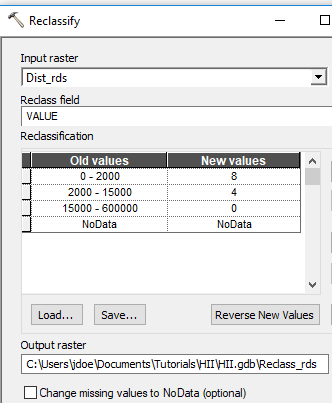
Click OK to accept the changes.
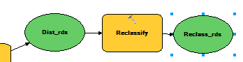
You may note that a line gets added in the model linking the output of a Euclidean Distance process to the newly created Reclassify process.
At this point, it’s a good idea to save the model once again by clicking on the model’s Save button.
You now need to add seven more reclassification tools. You will set each tool’s parameters as follows:
NOTE: Some NoData are reclassified as 0 so double-check your work!
|
Reclassify # |
Input |
Reclass Field |
Old values --> New values |
Output raster |
|
# 2 |
|
Value |
0 - 0.5 --> 0 |
.\HII.gdb\Reclass_dens |
|
# 3 |
|
Value |
0 - 2000 --> 8 |
.\HII.gdb\Reclass_rail |
|
# 4 |
|
Value |
0 - 15000 --> 4 |
.\HII.gdb\Reclass_riv |
|
# 5 |
|
value |
0 - 15000 --> 4 |
.\HII.gdb\Reclass_coast |
|
# 6 |
|
Value |
0 --> 0 |
.\HII.gdb\Reclass_lights |
|
# 7 |
|
Value |
1 --> 0 |
.\HII.gdb\Reclass_LC
|
|
# 8 |
|
Value |
0 – 30 --> 10 |
.\HII.gdb\Reclass_Urb |
At this point, you may notice the different symbols
preceding the input layers. The ‘recycling’ symbol ![]() indicates that the
layer currently does not exist in the TOC but will be made available from
another geoprocess in the model (Euclidean Distance in this exercise). The
‘layer’ symbol
indicates that the
layer currently does not exist in the TOC but will be made available from
another geoprocess in the model (Euclidean Distance in this exercise). The
‘layer’ symbol ![]() indicates that the
layer currently exists in the TOC and will NOT be derived from another
geoprocess in the model.
indicates that the
layer currently exists in the TOC and will NOT be derived from another
geoprocess in the model.
Save the HII model but keep the model window open.
Finally, we need to combine the scores or index values into a comprehensive HII value for each pixel. To complete this task, we will simply sum all the reclassified rasters.
In ArcToolbox, expand the Map Algebra toolset and drag-and-drop the Raster Calculator tool into the HII model.
Double-click the HII model’s Raster Calculator tool.
Sum all eight reclassified layers. It’s best that you double-click on each layer listed in the upper left window pane to copy its name into the expression box instead of manually typing it to avoid typos. Your expression should look something like,
"%Reclas_rail%" + "%Reclass_riv%" + "%Reclass_coast%" + "%Reclass_lights%" + "%Reclass_LC%" + "%Reclass_Urb%" + "%Reclass_rds%" + "%Reclass_dens%"
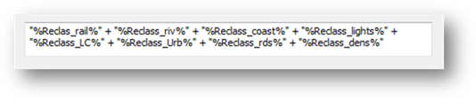
Name the output raster HII.
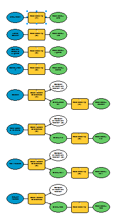
Your final model should look like this:
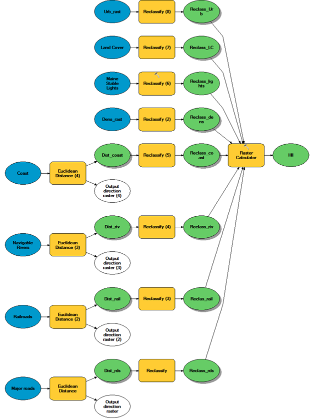
Save the model.
You are done creating the model. Now you will run the model to create the final output.
In the Model window, click on the Run icon ![]() (upper right-hand
side of the toolbar).
(upper right-hand
side of the toolbar).
A Model status window will pop-up indicating the geoprocess status.
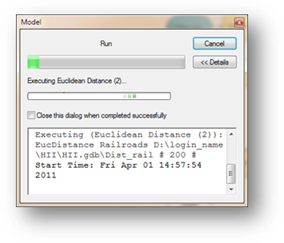
When all geoprocesses are finished, you will notice "shadows" cast by each geoprocess in the ModelBuilder window. This indicates that the model has finished processing the "shadowed" geoprocess.
If the HII model status window is not closed, but indicates that the model execution is complete, close the status window.
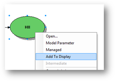
You will now add the final HII raster layer to the map document.
Right-click on the HII output and select Add to Display.
In ArcMap's TOC, turn off all layers except for the HII layer.
In the TOC, Double-click on the HII layer to access its Properties.
In the Layer Properties window, click on the Symbology tab.
Change the color ramp to one that ranges from red to green.
Check the Invert box to switch color order.
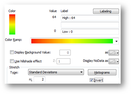
Click OK to close the Layer Properties window.
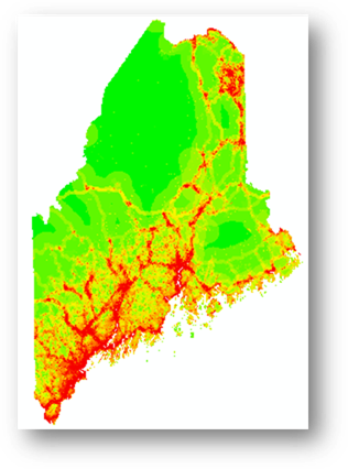
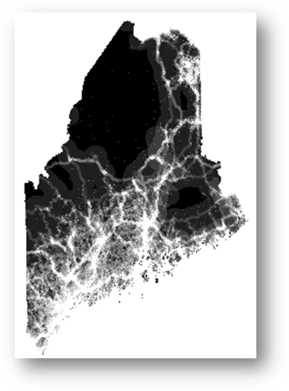
The HII values should range from 0 to 64. If not, there is a good chance that you did not properly specify at least one reclassification parameter. Go back to Step 6 and check that the reclassification values in your model match those listed in the table.
The ability to change just one parameter and have the software rerun all geoprocesses for you is one advantage of creating a model. Without a model, had you made a mistake early on in the workflow, you would have had to painstakingly rerun all subsequent geoprocesses one process at a time.
Another advantage to creating a geoprocess model is the ability to port it to different map projects and datasets. The model can be accessed from within any new map document.
Note that models can always be edited by right-clicking the model and selecting Edit.
Feel free to change the influence scores of the various variables in the reclassification processes and rerun the model.
Do you have other datasets you want to run through the HII model? Load the layers into your map document and substitute the layers used in this exercise with your layers.
References:
Sanderson, E.W., M. Jaiteh, M.A. Levy, K.H. Redford, A.V. Wannebo, and G. Woolmer. 2003. The Human Footprint and The Last of the Wild. BioScience 52, no.10 (October 2002): 891-904
![]() Manuel Gimond, last modified 7/12/2018
Manuel Gimond, last modified 7/12/2018