Downloading and mapping Census data
|
Create a folder called Census1 somewhere under your personal directory (e.g. C:\Users\jdoe\Documents\Tutorials\Census1). · Note that there are no files to download for this exercise. You will be provided instructions on how to download census data from the Census Bureau’s website in later steps. · Also note that a professional subscription to the socialexplorer.com website may be needed to download the data. If you are on a Colby College network, you should have full access to socialexplorer.com. |
In this exercise, you will learn how to query, download and map census data. You will use 2010 American Community Survey (ACS) data which is a sample survey collected continuously between decennial censuses.
This tutorial assumes that you have some familiarity with Excel.
Step 1: Open Social Explorer website
Step 2: Selecting the spatial extent
Step 3: Selecting and downloading census attributes
Step 4: Modifying the census data table in Excel
Step 5: Downloading Census shapefile
Step 6: Loading the census table and shapefile in ArcMap
Step 7: Joining non-spatial census table to a spatial layer
Step 8: Symbolizing the shapefiles by census data
In a browser, open the website http://www.socialexplorer.com/.
Note that certain services are only accessible via a subscription. Colby has a “professional access” subscription which offers unfettered access to census data.
Click on the Tables tab.

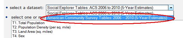
Next, expand the American Community Surveys (5-Year Estimates).
Click on Begin Report link next to American Community Survey (ACS) 2006--2010 (5-Year Estimates).
This places you in the data query environment.
You will download educational attainment data for each county in the US in a tabulated form. In subsequent steps, you will join this table to a shapefile of the US counties. Note that you can download data aggregated down to the census block-group level with the ACS 2006-2010 census data.
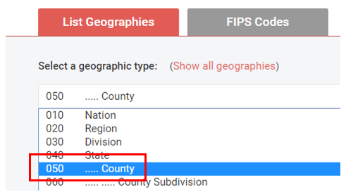
Under select a geographic type select County.
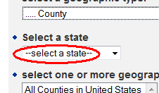
Do not change the select a state option. However, if you wanted to restrict the analysis to a single state, you would define the state in this step.
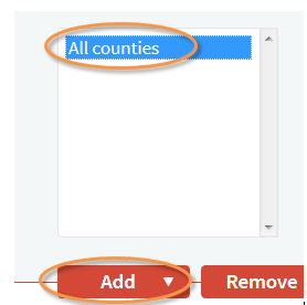
Under select one or more geographic areas, select All Counties then click on the Add link just beneath the selection window.
Your geographic query window should look something like this:
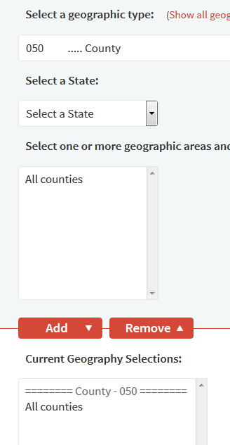
Click on Proceed to Tables to proceed to the attribute selection step.
The Social Explorer website provides you with both the original census data tables and a ‘filtered’ version of these data tables. The census ACS dataset is based on sample surveys (and not total enumeration) and is therefore an estimate of the total population. The Census bureau provides an estimate of the error along with its dataset. The filtered version of the tables excludes the margin of error (MoE) data. It’s always good practice to work with both the estimate and the MoE data, so in keeping with good practice you will choose to select the original census data table (note that this tutorial will not make use of the MoE).
To the right of the select a dataset field, choose American Community Survey Tables: 2006—2010.
Next, you will select the attribute associated with educational attainment.
Search for table B15002 (Sex by educational attainment for population 25 years and over) then add it to the Table Selections window.
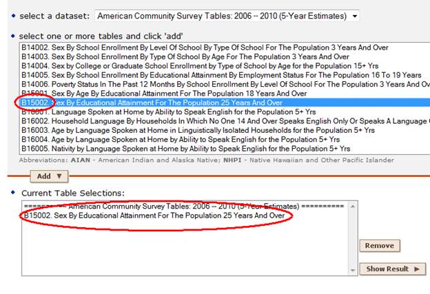
Click on Show Result to proceed to the next page.
On the next page, select the Data Download tab.

Click on the County data (CSV) link to download the data.
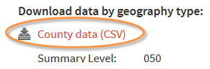
Note the file name you are downloading! You will need this information when searching for the file in the Downloads Folder on your PC.
If prompted, select to have the file saved to your hard disk.
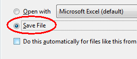
If you are downloading the file using Firefox, the file will most likely be saved under C:\Users\login_name\Downloads by default. You will want to copy that file to your project folder.
You will also want to download the data dictionary which provides descriptive information on the table’s attribute values.
Click on the Data dictionary link near the bottom of the page.
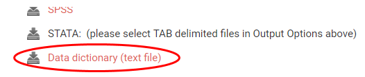
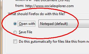
If prompted, select the Open with Notepad option.
The column (attribute) information for your dataset is defined in this file.
Make sure to save the data dictionary file in your project folder for future reference.
The file you downloaded from the Social Explorer website is in a comma delimited (CSV) file format. The file name is randomly generated so the filename shown in this tutorial will not necessarily match that of the file you downloaded.
A CSV file can be opened in either Excel or ArcMap. If data manipulation is needed before joining to a GIS layer, it is best to accomplish this in Excel.
Locate the CSV file you downloaded (if you use Firefox, this should be under C:\Users\login_name\Downloads) and open it with Excel.
You’ll note that the file has many columns (attributes). To decipher the column names, you will need to refer to the data dictionary file you downloaded in the previous step.
The data columns are broken down into three groups:
· Ancillary geographic data information (IDs and locations for the most part)
· Count data for each educational attainment/gender combinations
· Error estimates for each educational attainment/gender combinations
For this tutorial, we will focus solely on the count data for education attainment. The error data will not be used.
Column ACS_10_5yr_B15002001 (or simply B15002001 in the data dictionary file) represents total population 25 years or older for each county. This value will be used to normalize population having attained a bachelor’s degree or greater.
In Excel, for each county, you will sum all members of the population having a bachelor’s degree or greater for both the male and female population, then divide this sum by the total population giving you the fraction of the population having attained at least a bachelor’s degree. The algebraic expression looks like this:
![]()
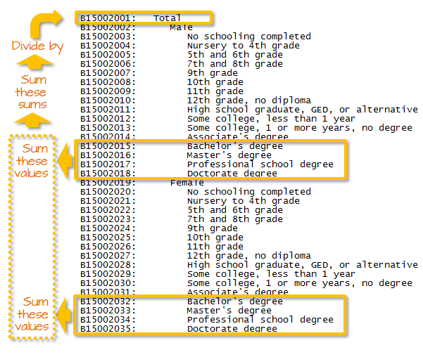
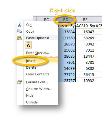
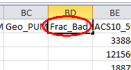
In Excel, you will create a new column to the left of the ACS10_5yr_B15002001 column. This column will be populated with the fraction of individuals having attained a bachelor’s degree or greater.
Right-click on the ACS10_5yr_B15002001 column tab and select insert.
Name the new column Frac_Bac (make sure not to have a space in the header name).
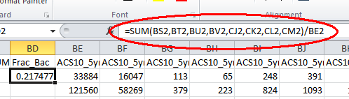
In the cell just beneath the header cell (in this working example, row 2 and column BD), type the algebraic expression for the fraction of the population having a Bachelor’s degree or greater. The expression might look like this,
= SUM(BS2,BT2,BU2,BV2,CJ2,CK2,CL2,CM2) / BE2
where BS2, BT2, etc… are the cell values associated with census variables B15002015, B15002016, etc… on row 2 (don’t forget to type the equal sign in the expression box!).
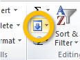
You can copy the formula in row 2 to all other rows in the Frac_bac column by selecting Frac_bac’s row 2 cell, clicking and holding the Shift key, and selecting the last (bottom) cell in the column. Then, in the Home ribbon near the top-right of the Excel window, click on the Fill (down) icon.
This should populate all cells in the Frac_bac column with unique values for each county.
If you are struggling with this step, you might want to read through this Microsoft Excel help page.
Save your Excel spreadsheet to a new Excel file under your Census1 project folder. Name the new Excel file census.xlsx.
Once saved, make sure to close the Excel file.
In the following step, you will download the shape file that delineates the US county boundaries.
In a web browser, navigate to the Census Bureau’s Tiger shapefiles website: https://www.census.gov/cgi-bin/geo/shapefiles/index.php.
From the Select a layer type pull-down menu, select Counties (and equivalent).
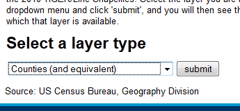
Click submit.
On the next web page, select All states in one national file in the County and Equivalent (2010) field, then click Download.
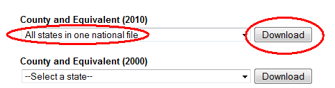
Unzip and save the contents of the file to your Census1 workspace (the file is just over 70 MB in size and may therefore take up to a minute or two to download).
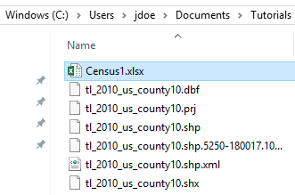
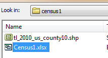
The spatial dataset is in a shapefile format, hence you will note the many files (all constituting a shapefile) extracted to your folder.
At this point, your Census1 folder may look like this:
If you are new to ArcMap, it is strongly suggested that you work through the Exploring a GIS map tutorial.
Open the ArcMap application.
Open a new (blank) ArcMap document.
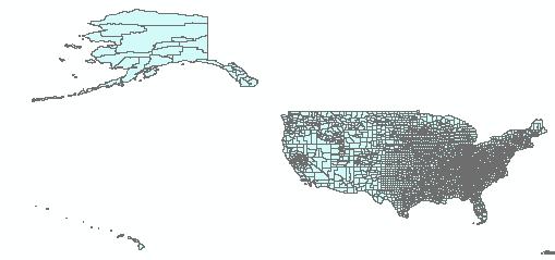
Load the tl_2010_us_county10 shapefile into your new map document.
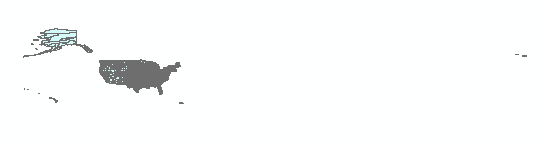
You’ll note that US territories (non-states) are also represented in the shapefile.
Zoom in on the 50 states.
Next, you will load the Excel file you recently created. ArcMap can only load one Excel sheet at a time. For more information on loading non-spatial data tables in ArcMap see the Joining Tables to Maps tutorial.
In your ArcMap document, click on the Add Data
button ![]() .
.
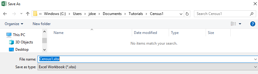
Double-click the Census1.xlsx file (in the Census1 folder).
This will display the lone Excel sheet in our Excel file (note that your sheet name may differ from the one displayed here).
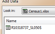
Select the sheet then click Add.
You should now see the spreadsheet in your TOC.
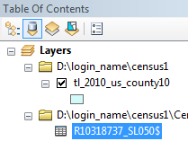
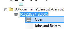
In the TOC, right-click on the spreadsheet and select Open.
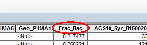
Scroll across the table, you should see the Frac_Bac column you created in the previous steps.
In the next section, you will learn to join this table to the counties shapefile.
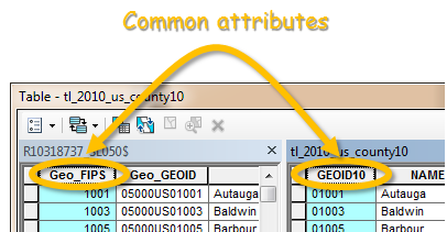
The census table will be joined to the shapefile using a common key (i.e. a common attribute). The census tables’ Geo_FIPS will be joined to the shapefile’s GEOID10 column.
However, there is a problem. Even though the values in both fields are the same, the data type for those attributes are different. The shapefile’s GEOID10 field stores the values as text while the Excel file’s Geo_FIPS field stores the values as numbers.
To circumvent this problem, you will create a new numeric field in the shapefile and convert the text values to numeric values.
Open the shapefile’s attribute table (if not already open).
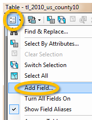
From the Table Options pull-down menu, select Add Field.
Name the new field GeoFIPS and set the data type to long integer.
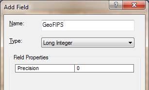
Click OK.
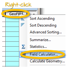
Right-click on the newly created field and select Field Calculator.
In the Field Calculator window, set the GeoFIPS field equal to [GEOID10]. This can be accomplished by typing the variable (with brackets) or by selecting and double clicking the field GEOID10 from the list of Fields.
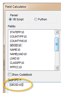
There is no need to add a text-to-number conversion function to the expression. ArcMap will perform the data type conversion automatically.
Click OK.
Next, you will perform the table-to-shapefile join.
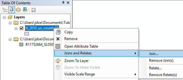
In the TOC, right-click on the shapefile tl_2010_us_county10 then select Joins and Relates >> Join.
Populate the fields as shown below (note that your spreadsheet name may differ from the one shown in this example).
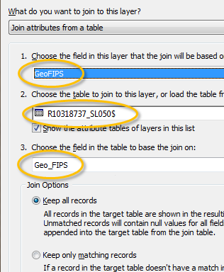
Click OK to perform the Join.
After the join, the content of the Excel spreadsheet gets appended to the tl_20120_us_county10 layer. Note that this join only exists in the current map document session. If a permanent join is desired, export the layer to a new feature class or shapefile (see Step 4 in the Joining Tables tutorial for more step-by-step instructions on exporting layers to a new data file).
In this last step, you will symbolize the counties shapefile using the Frac_bac attribute you computed in the Excel file.
Right-click on the shapefile layer and open its Properties window.
Select the Symbology tab, then Quantities. Select Frac_bac as the Value to symbolize.
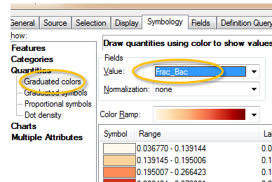
Click OK to see the results in the data view window.
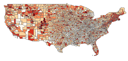
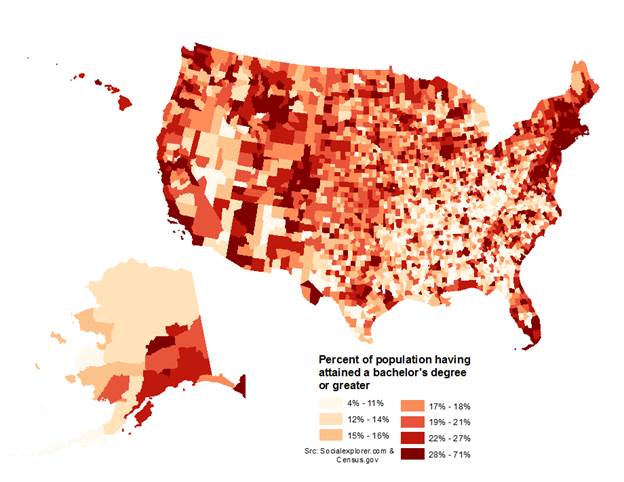
Feel free to glean inspiration from the Symbolizing Features tutorial to come up with a final map output.
Save your map document and close ArcMap.
This ends this exercise.
![]() Manuel Gimond, last modified on 7/11/2018
Manuel Gimond, last modified on 7/11/2018