Modeling hydrologic basins and flow
paths
|
1. Create a folder called Hydro somewhere under your personal directory (e.g. C:\Users\jdoe\Documents\Tutorials\Hydro\). 2. Download the data for this exercise then extract the contents of Hydro.zip into your newly created Hydro directory. |
In this exercise, you will learn to generate flow paths and hydrologic basins from an elevation raster. This tutorial requires that you enable the Spatial Analyst extension under Customize >> extensions.
Step 1: Smoothing
the elevation surface
Step 2: Creating a flow direction raster
Step 3: Creating a flow accumulation raster
Step 4: Identifying potential streams
Step 5: Delineating hydrologic basins
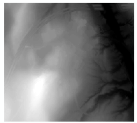
Open the Hydro.mxd document.
The map document consists of a Lidar derived raster elevation model of the Colby campus.
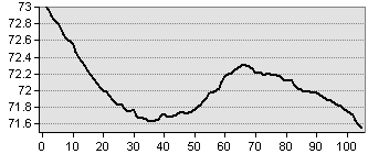
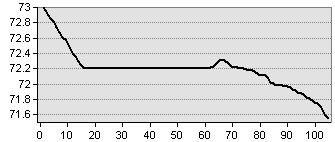
The first step is to remove isolated depressions from the elevation raster. This is needed to ensure that flow models reflect general topography and localized topography. For example, the following profile shows a localized depression (Figure 1) and its filled counterpart (Figure 2).
|
Figure 1 Original
profile |
Figure 2 Filled depression |
We’ll make use of the Fill tool which will identify and fill isolated depressions in the elevation layer.
In your Toolbox ![]() ,
open Spatial Analyst Tools >>
Hydrology >> Fill.
,
open Spatial Analyst Tools >>
Hydrology >> Fill.
Select Elev.tif as the input surface raster. Name the output Elev_fill.tif.

Click OK to run the geoprocess.
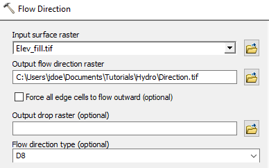
Next, we’ll create a flow direction raster. This layer will assign, for each pixel, a flow direction to its steepest downslope neighboring pixel.
In your Toolbox ![]() ,
open Spatial Analyst Tools >>
Hydrology >> Flow Direction.
,
open Spatial Analyst Tools >>
Hydrology >> Flow Direction.
Use Elev_fill.tif as the input raster, name the output Direction.tif and adopt the D8 flow direction type.
Click OK to run the geoprocess.
Each pixel is assigned an integer value that defines the flow direction. The following diagram matches the integer value to its flow direction.

Next, we’ll create a raster from the flow direction layer that computes the total number of pixels that feed into each pixel.
In your Toolbox ![]() ,
open Spatial Analyst Tools >>
Hydrology >> Flow Accumulation.
,
open Spatial Analyst Tools >>
Hydrology >> Flow Accumulation.
Use Direction.tif as the input raster, name the output Accumulation.tif and set the output data type to Integer.
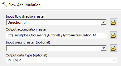
Click OK to run the geoprocess.
When possible, it’s good practice to seek the smallest data type needed for a file. Here, we are tallying the number of cells that feed into another which results in count values that are whole numbers (not fractions). This explains the choice of an integer raster for our output.
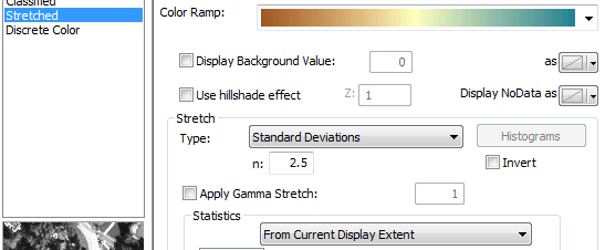
At first glance, the raster may look homogeneous. This is because the raster’s data values are skewed towards higher values.

You can change the symbology to reveal the distribution of values using the following template as an example (note the use of From Current Display Extent option under the Statistics block; this rescales the range of colors to the viewing extent).
Now zoom in on the raster to reveal flow paths.
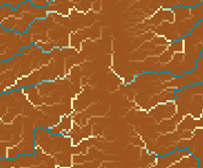
A pixel value of 0 indicates that no other pixel in the raster flows into it. A value of 1 indicates that 1 pixel flows into it. A value of 2 indicates that 2 pixels flow into it, etc… These values can be translated to watershed areas feeding into each pixel. Simply multiply the pixel value by the pixel’s surface area. In this example, the pixel size is 1 m² so a pixel whose accumulation value is 125,113 services an area of 125,113 x 1 m² = 125,113 m².
In this step, we’ll create a vector layer that identifies potential streams/rivers based on a defined accumulation value cutoff. Note that accumulation value alone is not enough to assess presence/absence of a flowing water body; other factors such as soil type and surface characteristics would be needed to make such a prediction.
In this example, we’ll create a stream/river vector layer from all accumulation pixels whose value is greater than 200,000 (i.e. the pixel services an area of 200,000 m² or greater).
In your Toolbox ![]() ,
open Spatial Analyst Tools >> Map
Algebra >> Raster Calculator.
,
open Spatial Analyst Tools >> Map
Algebra >> Raster Calculator.
Type the following expression in the expression box and name the output acc_200k.tif.
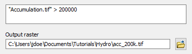
Click OK to run the geoprocess.
The output is a binary raster where the value of 1 indicates that the pixel has an accumulation value greater than 200,000 and a value of 0 indicates that the pixel has an accumulation value less than or equal to 200,000.
The raster representation of the drainage areas can be difficult to visualize because of the small pixel size. We’ll therefore convert the raster to a polyline whereby the pixels with values of 1 will be converted to line segments.
In your Toolbox ![]() ,
open Conversion Tools >> From
Raster >> Raster to Polyline. Set acc_200k.tif
as the input raster and name the output shapefile Drainage.shp.
,
open Conversion Tools >> From
Raster >> Raster to Polyline. Set acc_200k.tif
as the input raster and name the output shapefile Drainage.shp.
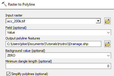
Click OK to run the geoprocess.
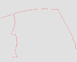
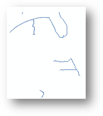
You now have a vector representation of the streams.
Finally, you will identify all drainage basins using the directions raster layer.
In your Toolbox ![]() ,
open Spatial Analyst Tools >>
Hydrology >> Basins. Set Direction.tif as the input raster and Basins.tif as the output raster.
,
open Spatial Analyst Tools >>
Hydrology >> Basins. Set Direction.tif as the input raster and Basins.tif as the output raster.
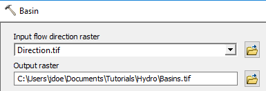
Click OK to run the geoprocess.

You can create a polygon version of the layer using the Raster to Polygon tool.
In your Toolbox ![]() ,
open Conversion Tools >> From
Raster >> Raster to Polygon. Set acc_200k.tif
as the input raster and name the output shapefile Drainage.shp.
,
open Conversion Tools >> From
Raster >> Raster to Polygon. Set acc_200k.tif
as the input raster and name the output shapefile Drainage.shp.
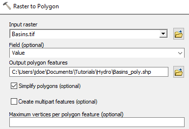
Click OK to run the geoprocess.
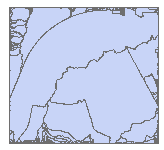
You’ll note the many small polygons near the edge of the study extent. Many of these polygons probably belong to the same basin but because the direction raster is restricted to the edge of this study extent, only those (exposed) flow direction pixels at the edge are used to define individual basins. For example, the following direction raster grid suggests a single basin (all pixels end up flowing to the upper left-hand corner).
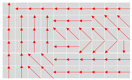
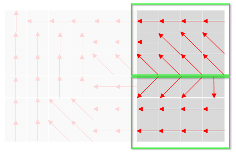
If the study extent was limited to the four right most set of pixel columns, then two separate basins would be identified.
© Manny Gimond,