Image Processing
|
1. Create a folder called Image_process. On DIA 322 computers, you might want to create this folder in your user Documents folder (e.g. C:\Users\jdoe\Documents\Image_process). On the DIA 222 computers, you might want to create this folder on the D: drive under D:\course number\user name\ (e.g. D:\ES212\jdoe\Image_process). 2. Download the data for this exercise and uncompress the contents of Image_process.zip file to your newly created Image_process directory. |
Remote sensing makes it possible to survey larger areas, in less time, and with fewer resources than could be accomplished by surface study. Images generated by sensors aboard aircraft or satellite platforms can be used to study aquatic or terrestrial productivity, phytoplankton community species composition, wetlands, geology, surface temperatures, wildfires, sea ice, landforms, and much more. The information contained in these images is not immediately interpretable, however, and some training is necessary in order to interpret the many different types of images.
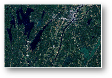
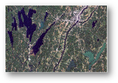
In this exercise you will use satellite imagery of the Waterville area acquired from the Landsat 7 ETM+ satellite on 9/10/2002. The Landsat 7 ETM+ satellite generates and makes available imagery taken by imaging sensors orbiting about 700 km above the earth surface. The Enhanced Thematic Mapper (ETM+) on Landsat has a resolving power of about 30 meters and can distinguish features on the earth's surface 30 meters apart. It requires 233 orbits over a period of 16 days to cover most of the earth surface. Each image is almost square and covers approximately 10,000 square miles of the planet's surface.
You will experiment with ArcGIS’ supervised and unsupervised classification tools and attempt to extract 5 distinct land cover classes. The Spatial Analyst extension is needed to access the classification tools.
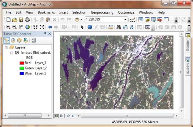
Step 1: Open Landsat 7 ETM+ data in ArcMap
Step 2: Displaying different band combinations
Step 3: Creating a visually enhanced raster using a panchromatic band
Step 4: Unsupervised classification
Step 5: Supervised classification
Step 6: Optional exercise: classify a GeoEye-1 satellite image
Click on the Windows icon ![]() in
the lower left-hand corner of your desktop, click on All Programs, expend the ArcGIS folder and click on ArcMap 10.X.
in
the lower left-hand corner of your desktop, click on All Programs, expend the ArcGIS folder and click on ArcMap 10.X.
In the ArcMap – Getting Started window, click on Browse for more. A file management window will pop-up. Navigate to your data folder (e.g. D:\login_name\Image_process\) and open Map.mxd.
Next, you will enable the Spatial Analyst extension that will allow us to use the image classification functions.
In the main menu, go to Customize >> Extensions.
If not already checked, check off the Spatial Analyst extension.
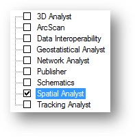
Click Close to close the Extensions window.
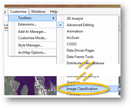
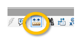
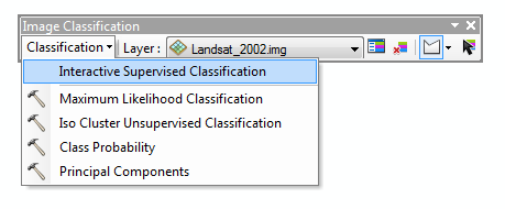
Next, you will launch the Image Classification toolbar. You will use functions from this toolbar to classify images in later steps.
In the main menu, go to Customize >> Toolbars and select Image Classification.
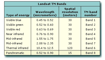
There are different bands that comprise the Landsat 7 ETM+ raster data. Each band covers a different bandwidth and is, thus, extracting different information from the same location. Refer to the following table for a description of each band.
The 2002 Landsat layer in the TOC does not have the Panchromatic band. It is stored as a separate file in your project folder because of its finer spatial resolution. You will add this layer separately in a later step.
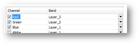
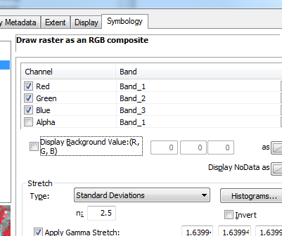
You can choose which bands to assign to the display’s red, green and blue channels.
Right-click on Landsat's layer in the TOC and select Properties.
Select the Symbology tab.
Assign different bands (identified as Layer_XX in the band selection window) to each Red, Green and Blue Channels and observe the result in the Data View window.
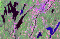
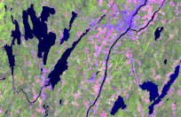
Here are a few band combination examples:
|
Band combinations |
Resulting image |
|
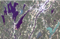
R= 3, G = 2, B = 1 · Creates a 'natural color' image from the visible bands
|
|
|
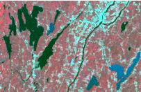
R = 4, G = 3, B = 1 · Detailed vegetation and crop analysis · Wetland studies · Urban development and land use studies
|
|
|
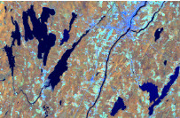
R = 4, G = 5, B = 3 · Analysis of soil moisture and vegetation conditions · Location of inland water bodies and land/water boundaries |
|
|
R = 7, G = 4, B = 2 · Analysis of soil and vegetation moisture conditions · Location of inland water · Vegetation appears in shades of green |
|
|
R = 5, G = 4, B = 3 · Separation of urban and rural land use · Identification of land/water boundaries |
|
|
R = 4, G = 5, B = 7 · Detection of clouds, snow, and ice · Especially used in high latitudes |
|
When done experimenting with the different band combinations, revert back to a 3, 2, 1 band combination (i.e. the ‘natural colors’ bands).
Using the zoom tool, zoom in on the image until individual pixels become distinguishable from one another.

Select the measure tool from the toolbar.
If the distance units are not in meters, change the measurement units to meters:
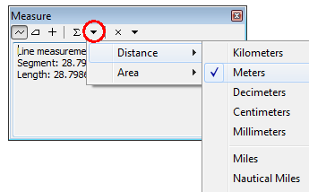
Measure the distance width of a pixel.
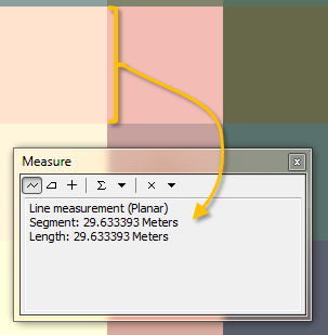
It should be approximately 30 meters making the cell area about 900 square meters.
Band 8 of Landsat produces an image with 15 meter pixels. You will merge this band with the ‘coarser’ bands to create a ‘visually enhanced’ raster.
Click on the Add
Data icon ![]() in
the toolbar.
in
the toolbar.
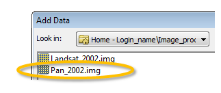
Expand the top folder connection in the Add Data window.
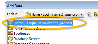
In the login_name\Image_process connection folder, add Pan_2002.img.
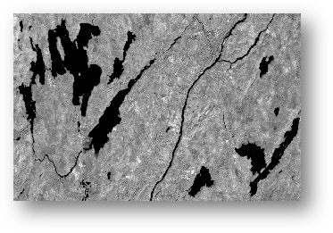
Because this is a single band layer, only grayscales are used to symbolize the panchromatic data.
Next, you will merge this panchromatic raster with the multiband Landsat_2002 layer to create a spatially enhanced raster layer.
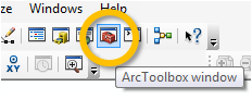
If the ArcToolbox is not already open, click on the Arctoolbox icon on the menu bar.
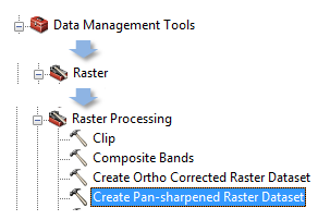
In the Toolbox expand Data Management Tools >> Raster >> Raster Processing and double-click Create Pan-sharpened Raster Dataset.
Before proceeding, it’s always helpful to understand what a geoprocessing tool does exactly. ArcGIS’ pan-sharpening tool uses the higher resolution panchromatic raster to estimate what a higher resolution multispectral raster would look like. Landsat’s panchromatic image spans three bands, the green red and near-infrared. It then follows that the radiometric intensity of the panchromatic band should be very close to the sum of the radiometric values of the three bands. However, the panchromatic band’s sensitivity to the three bands is not uniform as can be seen in the following figure:
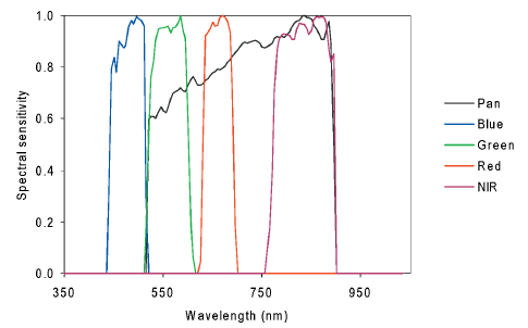
Source: Svab and Ostir (2006)
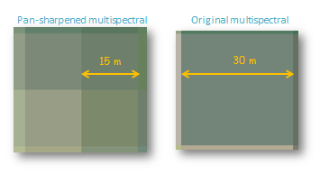
We can use this information to estimate what the green, red and near-infrared band values are at a smaller pixel size. The general idea behind this process is illustrated in the following graphic:
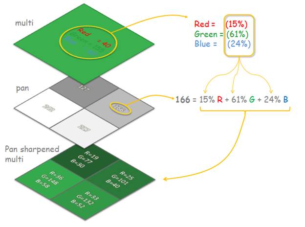
However, as noted earlier, the radiometric contribution of each band to the overall panchromatic signal is not uniform. This property of the panchromatic band can be taken into account by applying a weight to each band (see here for more detail).
NOTE: As of version 10.2, Arcmap seems to require that the pan sharpened output be saved in a geodatabase--saving the output as a .img or .tif file produces a raster of identical resolution to the input multi-band raster. In the following step you will be asked to save the output raster file to a geodatabase located in your working project folder.
In the Create Pan-sharpened Raster Dataset tool window, fill in the fields as illustrated below. Name the output PanSharp (save it in the Landsat.gdb). The weights entered in the last four fields reflect the sensitivity of the panchromatic band to the narrower bands (note that the blue band does not contribute to the panchromatic signal). Also, note that the band weights you will use differ from the default values assigned by ArcMAP.
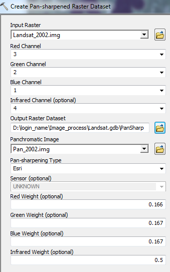
Click OK to run the geoprocess.
Zoom in on an area until individual pixels become distinguishable from one another.
Toggle back and forth between the pan-sharpened layer and the original multi-spectral layer. Note the difference in spatial resolution.
The new pan-sharpened raster may look grainy. To remedy this, you can change the layer’s properties by setting the Display parameters as shown in the next figure.
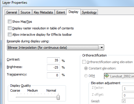
You might also want to change the Symbology stretch type to Standard Deviations.
Pattern recognition is the science—and art—of finding meaningful patterns in data, which can be extracted through classification. By spatially and spectrally enhancing an image, pattern recognition can be performed with the human eye; the human brain automatically sorts certain textures and colors into categories.
In a computer system, spectral (band) pattern recognition can be more scientific. Statistics are derived from the spectral characteristics of all pixels in an image. Then, the pixels are sorted based on mathematical criteria. The classification process breaks down into two parts: training and classifying (using a decision rule).
First, the computer system must be trained to recognize
patterns in the data. Training is the process of defining the criteria by which
these patterns are recognized. Training can be performed with either a
supervised or an unsupervised method.
Unsupervised training is computer-automated. It enables you to specify
some parameters that the computer uses to uncover statistical patterns that are
inherent in the data. These patterns do not necessarily correspond to directly
meaningful characteristics of the scene, such as contiguous, easily recognized
areas of a particular soil type or land use. They are simply clusters of pixels
with similar spectral characteristics. In some cases, it may be more important
to identify groups of pixels with similar spectral characteristics than it is
to sort pixels into recognizable categories.
Unsupervised training is dependent upon the data itself for the definition of
classes. This method is usually used when less is known about the data before
classification. It is then the analyst's responsibility, after classification,
to attach meaning to the resulting classes. Unsupervised classification is
useful only if the classes can be appropriately interpreted!
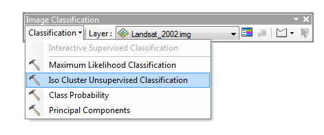
From the Image Classification toolbar (you should have added this toolbar in Step 1) select Classification >> Iso Cluster Unsupervised Classification.
In the Unsupervised Classification window, select landsat_2002.img as the input data layer (this is the original raster, not the pan-sharpened one), set the desired number of classes to 5, and set the output image to D:\login_name\RS2\unsup_class.img.
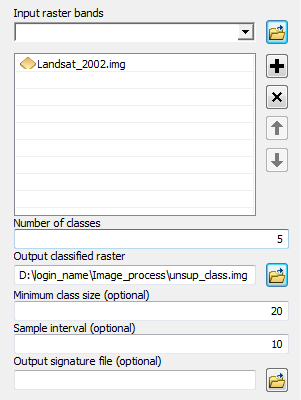
Click OK to run the classification geoprocess.
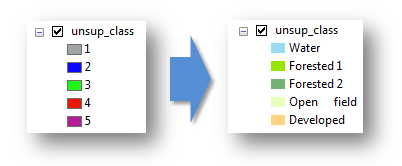
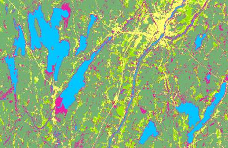
A new data layer will be added to your TOC. This layer is a discrete raster with 5 unique codes.
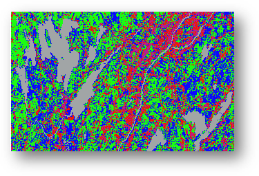
Attempt to identify the class types and assign a proper color scheme. You can change the color schemes and labels by double clicking on each individual color swatch of the unsup_class layer in the TOC.
Your classified rater may look something like this:
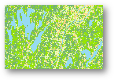
The unsupervised classification geoprocess does a decent job in discriminating between major categories such as water, urban and vegetation, but it seems to struggle in separating out the different vegetation (or ‘green’) categories. We can improve on this classification process by ‘training’ the classification tool using a priori knowledge of the underlying geographic features
In supervised training, you rely on your own pattern recognition skills and a priori knowledge of the data to help the system determine the statistical criteria (signatures) for data classification. To select reliable samples, you should know some information—spatial or spectral—about the pixels that you want to classify.
The location of a specific characteristic, such as a land cover type, may be known through ground truthing. Ground truthing refers to the acquisition of knowledge about the study area from field work, analysis of aerial photography, personal experience, etc. Ground truth data are considered to be the most accurate (true) data available about the area of study. Ideally, they should be collected at the same time as the remotely sensed data.
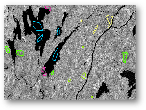
In the Image Classification toolbar, make sure that Landsat_2002.img is selected and click on Training sample manager.
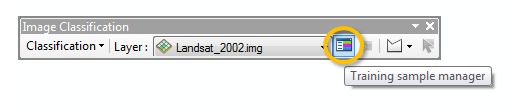
The Training Sample Manager window allows you to delineate and identify known features. The image classifier then uses this information to fine-tune its classification geoprocess.
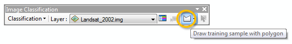
In the Image Classification toolbar click on the Draw training sample with polygon icon.
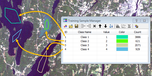
Next, draw a few polygons that delineate water bodies inside the scene. Make sure not to cover any land features.
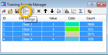
Next, selected all water polygons (while
holding and pressing the ctrl key) then click on Merge ![]() to
group all water polygons into a single class.
to
group all water polygons into a single class.
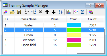
Name the new class water and assign it a blue color by clicking on its color swatch.
Follow these same steps to create urban, forest, open field and wetlands training samples.
Here’s an example of what your training sites might look like:
Next, from the Image Classification toolbar, select Interactive Supervised Classification.
You should notice an improvement in the overall classification.
Note that this can be an iterative process whereby you tweak the training classes as needed to improve upon each supervised classification process.
Feel free to modify/add training classes as needed. Don’t forget to rerun the classification after changing the classes.
The classified image resulting from the Supervised classification geoprocess is only a temporary layer inside the map document. If you want this layer to be a permanent raster, you need to export it.
Right-click on Classification_Landsat_2002.img and select Data >> Export Data.
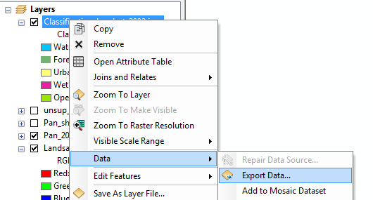
Set the output workspace to D:\login_name\Image_process (or wherever your working folder is located) and name the output sup_class.img (make sure to select IMAGINE as the data file format).
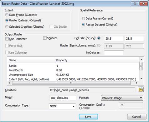
Click Save.
On your own, classify features in the GeoEye-1 satellite image subset. Note that GeoEye has fewer bands than Landsat, but it has a finer spatial resolution.
GeoEye data can be downloaded from here (save the data in your current project folder).
![]() Manuel Gimond, last modified on 8/22/2013
Manuel Gimond, last modified on 8/22/2013