Finding the least-cost path between two locations
|
1. Create a folder called Least_cost_path somewhere under your personal directory (e.g. C:\Users\jdoe\Documents\Tutorials\Least_cost_path). 2. Download the data for this exercise then uncompress the Least_cost.zip file to your newly created Least_cost_path directory. |
In this exercise, you will identify the most cost effective path between two locations based on elevation slope and landuse type.
You will need to enable Spatial Analyst extension to complete most of the steps in this exercise.
Step 1: Open the ArcMap document
Step 3: Reclassify the Slope Layer
Step 4: Reclassify Land Use Layer
Step 5: Create a Total Cost Layer
Step 6: Create a Cost-Distance and Cost-Direction layer
Step 7: Compute the Least Cost Path
Navigate to your Least_cost_path folder and open the Least_cost.mxd document in ArcMap.
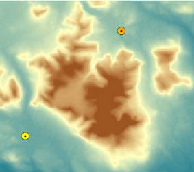
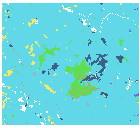
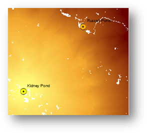
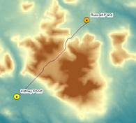
The map shows a section of Baxter State Park (Maine) that surrounds Mt. Katahdin. The two point features represent Kidney Pond and Russell Pond campsites (you might want to enable labeling for the two point layers).
The two other layers in the map document represent elevation (in meters) and land use. Both of these layers are rasters.
The purpose of this exercise is to find a path that links both campsites while minimizing the “cost” of travel (by foot). This cost (or impedance) is a factor of two variables: elevation slope and land cover. The steeper the slope or the denser the vegetation the more arduous the hike. We want to minimize this impedance, in other words we want to strike a balance between total distance walked and time spent overcoming obstacles.
This requires the creation of a “cost” layer that assigns a cost (or impedance) value for each pixel based on slope and land cover type. This cost layer will later be used to calculate a cost distance layer.
But first, we must create a slope raster layer.
In ArcToolbox, open Spatial Analyst Tools >> Surface >> Slope tool.
In the Slope tool window, select Elevation as the input raster, …\Least_cost_path\Slope.tif as the output raster and PERCENT_RISE as output measurement.
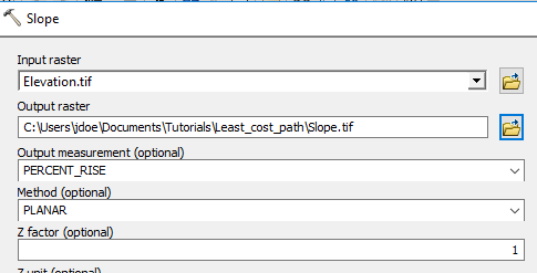
Note that if the elevation units were different from the horizontal units, a Z factor conversion would need to be applied. Since the Elevation layer you are using has vertical units of meters a conversion is not necessary (the horizontal units are also in meters).
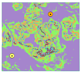
Click OK to run the geoprocess.
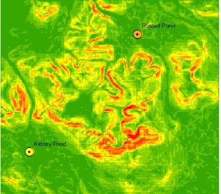
Steep areas are symbolized with a red hue.
Next, you will convert the percent rise values to unitless reclassified “cost” values.
In ArcToolbox open Spatial Analyst Tools >> Reclass >> Reclassify tool.
In the Reclassify tool window, set Slope as the input raster and Value as the reclass field.
You will use a standard classification scheme to recode the slope values.
Click on the Classify button.
Select Equal Interval as the classification method and choose to have the tool create 10 classes. Click the Tab key to ensure that the 10 classes are applied to the data.
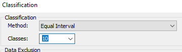
Click OK to close the Classification window.
Finally, set the output raster to …\Least_cost_path\RecSlope.tif.
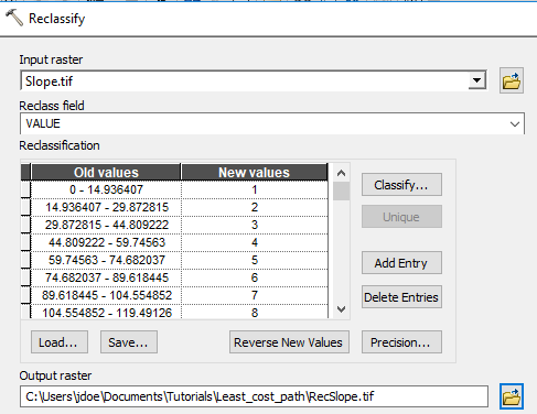
Click OK to run the Reclassify tool.
Next, you will reclassify the land cover layer to create another cost surface.
In ArcToolbox open Spatial Analyst Tools >> Reclass >> Reclassify tool.
In the Reclassify tool window, set LandUse as the input raster and Value as the reclass field.
This time, you will use a predefined classification scheme to recode the slope values.
Click on the Load... button in the Reclassify window.
Navigate to your working folder and select the lc_reclass table.
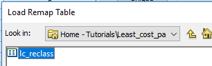
Click on the Load button to load the table into the reclassify tool.
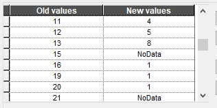
The table automatically populates the recode fields for you.
Finally, set the output raster to …\Least_cost_path\RecLandUse.tif.
Click OK to run the reclassify tool.
If you turn off all raster layers except the RecLandUse layer, you’ll note that several pixels have no data (they appear as transparent pixels in the map).
NoData pixels will tell the cost-path tool not to include them in the analysis. The NoData pixels were assigned to water bodies in the reclassify tool.
Now that we have created cost layers for slope and land use, we now must combine the two to create a total cost layer.
In ArcToolbox open Spatial Analyst Tools >> Map Algebra >> Raster Calculator tool.
In the expression window, type the following expression:
("RecLandUse" + "RecSlope") / 2
Set the output raster to …\Least_cost_path\Cost.tif.
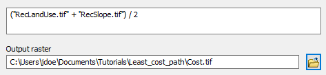
Click OK to perform the raster calculation.
Your new raster layer incorporates both impedance layers (slope and land cover). Note that all NoData pixels remain NoData in the output.
Naturally, you could have added a weight to one of the two layers. In fact, the reclassification scheme used in this exercise is subjective. More objective approaches in defining the cost from the slope and land use layers should be investigated.
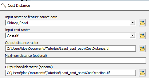
In ArcToolbox, open Spatial Analyst Tools >> Distance >> Cost Distance tool.
The feature source data is Kidney_Pond (this is the feature we are computing the cost-distance from)
The input cost raster is the Cost raster.
Set the output backlink raster to …\Least_cost_path\CostDirection.
The backlink (optional) output is the cost-direction output. We could have computed the cost-direction output separately using the Spatial Analyst Tools >> Distance >> Cost Back Link. In essence, we are saving an extra step here.
Before we run the tool, we need to tell ArcGIS that the new (to be created) raster’s extent should match that of the other rasters in the map document.
Click on the Environments button.
In the Environments Settings window, expand Processing Extent.
Set both the extent and the snap raster to Cost.
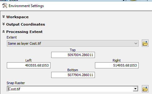
Click OK to close the Environment Settings window.
Click OK to run the Cost Distance tool.
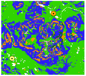
When the geoprocess completes, you will see two new raster layers in your TOC.
The CostDistance layer shows the cumulative cost distance from Kidney pond to all pixels within the extent. Both the slope and land use impedances influence the results.
The CostDirection layer shows, for each pixel in the extent, the direction to take to follow the least cost path back to Kidney Pond.
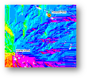
It is the cost direction layer that is used in the final step to find the least cost path from Kidney Pond to Russell Pond.
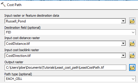
In ArcToolbox, open Spatial Analyst Tools >> Distance >> Cost Path tool.
In the Cost Path tool, set the feature destination to Russel_Pond.
Set the Input cost distance raster to CostDistance.
Set the Input cost backlink layer to CostDirection.
Set the output raster to LeastCostPath.tif in your project folder.
Click OK to run the analysis.
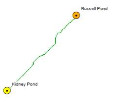
The LeastCostPath layer is a raster layer. It is close to a Euclidean distance except for a couple minor detours around wetlands (which were assigned a relatively high cost in this analysis).
To create a more aesthetically pleasing feature, you can convert the raster path to a vector path.
In ArcToolbox, open Conversion Tools >> From Raster >> Raster to Polyline tool.
Set the field parameters as follows:
· Input raster: LeastCostPath
· Field: Value
· Output polyline features: …\Least_cost_path\Path.tif
· Background value: NODATA
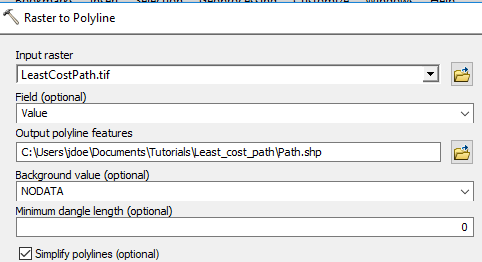
Click OK to convert the raster to a polyline.
The new feature is a vector layer.
This ends this exercise
![]() Manuel Gimond, last modified on 7/13/2018
Manuel Gimond, last modified on 7/13/2018