Vegetation Indices
|
1. Create a folder called NDVI. On DIA 322 computers, you might want to create this folder in your user Documents folder (e.g. C:\Users\jdoe\Documents\ NDVI). On the DIA 222 computers, you might want to create this folder on the D: drive under D:\course number\user name\ (e.g. D:\ES212\jdoe\ NDVI).
|
In this exercise, you will use ArcGIS’ Image Analysis tool
to compute Normalized Difference Vegetation Index (NDVI) values for the Howland
Forest area (located in Maine) using MODIS
(Moderate-Resolution Imaging Spectroradiometer) satellite data. You will then
use Spatial Analyst to compute zonal statistics for an area of interest.
NDVI is a vegetation index that is associated with vegetation density. It is
often used to distinguish vegetation from non-vegetation features. It
normalizes the difference between the green leaf scattering in the
near-infrared to the chlorophyll absorption. The NDVI is computed as follows:
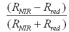
where RNIR is the reflectance in the near infrared part of the spectrum, and Rred is reflectance in the red part of the spectrum. The value of the index ranges from -1 to 1. A common range for green vegetation is 0.2 to 0.8.
Step 2: Calculating an NDVI value for the month of January
Step 3: Compute NDVI values for the other 11 months
Step 4: Averaging NDVI values within an area defined by a polygon
Step 5: Graphing the NDVI values
Navigate to your NDVI project folder and open the NDVI.mxd map document.
|
|
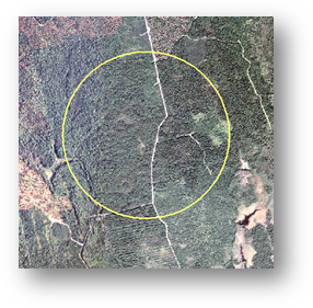
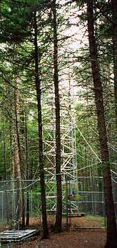
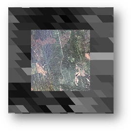
The yellow circle encompasses an area of the Maine Howland forest that is part of the AmeriFlux network. An instrumented tower is located at the center of the circle The tower provides continuous observations of ecosystem level exchanges of CO2, water, energy and momentum spanning various time scales. The Howland forest main tower site is managed by the USDA Forest Service, the Woods Hole Research Station, the University of Maine, the University of Georgia and the University of California. The forest surrounding the tower is composed of red spruce, eastern hemlock, other conifers such as balsam fir, white pine, northern white cedar, and hardwoods such as red maple and paper birch. A breakdown of each species follows: · 41% red spruce (Picea rubens Sarg.), · 25% eastern hemlock (Tsuga canadensis (L.) Carr.), · 23% other conifers (primarily balsam fir, Abies balsamea (L.) Mill., white pine, Pinus strobus L., and northern white cedar, Thuja occidentalis L.) and, · 11% hardwoods |
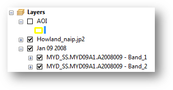
Turn off the Howland_naip layer and turn on the Jan 09 2008 group layer.
All 12 MODIS group layers in your map document are in a raster data format, yet they don’t seem to follow an orthogonal grid of cells that you might be accustomed to seeing. This is because the MODIS data were provided to us in a Sinusoidal projection which distorts shape in our area of interest. One could reproject the raster to a coordinate system better suited for the state of Maine however, in doing so, we risk ‘contaminating’ the original radiometric signal. This is because of the use of interpolation techniques that are needed to transform the raster from one coordinate system to another. We will therefore not reproject the MODIS rasters in this exercise.
A MODIS image is composed of different 'bands'. Each band has bits of information such as reflectance value for a particular bandwidth and solar zenith angle at the time of the image acquisition. The following table lists the bands and their description.
|
Band number |
Description |
UNITS |
MULTIPLY BY SCALE FACTOR |
|
1 |
500m
Surface Reflectance Band 1 |
Reflectance |
0.0001 |
|
2 |
500m
Surface Reflectance Band 2 |
Reflectance |
0.0001 |
|
3 |
500m
Surface Reflectance Band 3 |
Reflectance |
0.0001 |
|
4 |
500m
Surface Reflectance Band 4 |
Reflectance |
0.0001 |
|
5 |
500m
Surface Reflectance Band 5 |
Reflectance |
0.0001 |
|
6 |
500m
Surface Reflectance Band 6 |
Reflectance |
0.0001 |
|
7 |
500m
Surface Reflectance Band 7 |
Reflectance |
0.0001 |
|
8 |
500m Reflectance Band Quality |
Bit Field |
na |
|
9 |
Solar Zenith Angle |
Degree |
0.01 |
|
10 |
View Zenith Angle |
Degree |
0.01 |
|
11 |
Relative Azimuth Angle |
Degree |
0.01 |
|
12 |
500m State Flags |
Bit field |
na |
|
13 |
Day of Year |
Julian day |
na |
Only bands 1 and 2 (representing the red and near-infrared parts of the spectrum) are present in this map project for each month of the year 2008. The bands are grouped by month.
In this exercise you will use bands 1 and 2 to compute the NDVI values for each pixel in the MODIS rasters.
To calculate the NDVI value, you will need to activate the Spatial Analyst extension.
From the Customize pull-down menu select Extensions.
Turn on the Spatial Analyst extension by checking the box next to the extension.
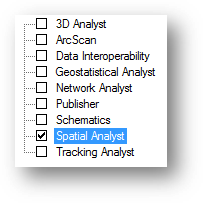
Click Close to close the Extensions window.
If not already opened, open the Toolbox by clicking
on the Toolbox button![]() .
.
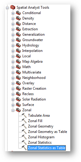
In ArcToolbox, expand Spatial Analyst Tools >> Map Algebra.
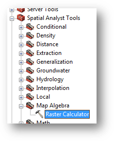
Double-click on the Raster Calculator tool.
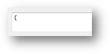
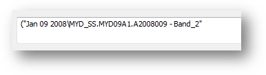
In the Raster
Calculator window, click on the open parenthesis symbol
![]() .
.
This action will add the parenthesis symbol to the expression window.
Next, double-click
on ![]() .
.
This will add Band 2 from the Jan 09 data set to the expression window.
Next, Click
(single click) on the minus operator ![]() to add it to the expression window.
to add it to the expression window.
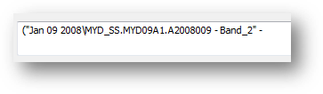
Next, double-click
on ![]() .
.
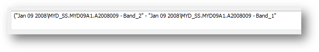
Next, click on
the close parenthesis symbol ![]() .
.
At this point, you have
defined the numerator ![]() for the NDVI
formula.
for the NDVI
formula.
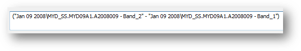
On your own, complete
the expression by adding the denominator ![]() component of the NDVI formula (don’t forget to add the ‘divide by’
operator).
component of the NDVI formula (don’t forget to add the ‘divide by’
operator).
When done, your expression box should look like this:

There is yet one more addition to the expression that will be needed to compute the NDVI: the Float function. All MODIS layers are of integer type. This means that the output of an algebraic expression will also be an integer even if a fraction is present in the expression. For example, the fraction 245/340 will result in an output value of 0 (value is rounded down). If a float output is desired, adding the Float function to the numerator or denominator will be required such as Float(245)/340.
In the expression box, add the Float function in front of the first parenthesis by typing ‘Float’.
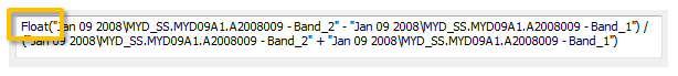
The expression now looks like this:
Float("Jan 09
2008\MYD_SS.MYD09A1.A2008009 - Band_2" - "Jan 09
2008\MYD_SS.MYD09A1.A2008009 - Band_1") /
("Jan 09 2008\MYD_SS.MYD09A1.A2008009 - Band_2" + "Jan 09
2008\MYD_SS.MYD09A1.A2008009 - Band_1")
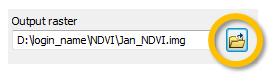
Finally, set the output path and raster name to …\NDVI\Jan_NDVI.img (you might want to click on the folder icon to set the directory path and define the filename—don’t forget to add the .img extension).
Click OK to run the geoprocess.
When the geoprocess is complete, a new raster layer will be added to the TOC.
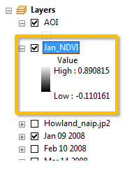
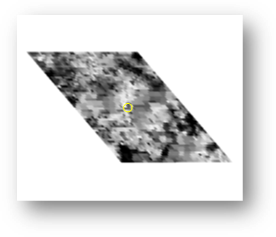
The output image represents NDVI values for each pixel. The greater the value (i.e. the closer the value is to 1), the ‘greener’ the biomass within the pixel.
So far, you have only computed an NDVI raster for the month of January.
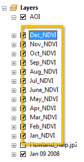
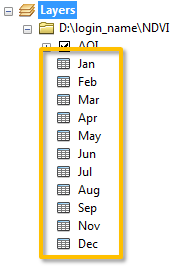
On your own, repeat the procedure outlined in step 2 to create NDVI rasters for the remaining 11 months. Name the output rasters Feb.NDVI.img, Mar_NDVI.img, etc…
When complete, you should see 12 NDVI rasters in your TOC.
You are interested in finding the average NDVI value surrounding an instrumented tower in the Howland forest. The area encompassing the tower is represented by the data layer AOI .
One way to average the NDVI values within an area of interest is to use the Identify tool to read each pixel's NDVI value then compute the average. This may be a time consuming process, especially if you need to perform this task for all 12 NDVI data layers. Fortunately, ArcGIS provides us with a tool that computes an average value for all pixels falling within an area of interest.
In the ArcToolbox menu tree, navigate to Spatial Analyst Tools >> Zonal and select Zonal Statistics as Table.
In the Zonal Statistics as Table window select AOI as the 'Input raster or feature zone data' value, Id as the zone field, Jan_NDVI as the input value raster and …\NDVI\Jan.dbf as the output table (don’t forget to add the .dbf extension).
Set the Statistics type to MEAN.
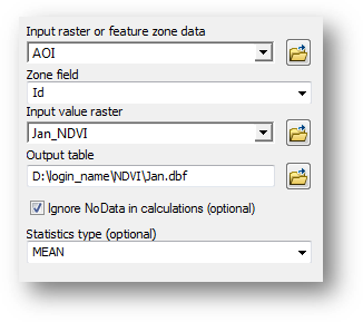
Click OK to run the geoprocess.
The newly created Jan table will be added to your TOC.
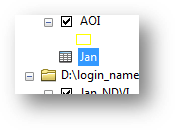
Right-click on Jan and select Open.
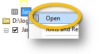
This brings up the attribute table.
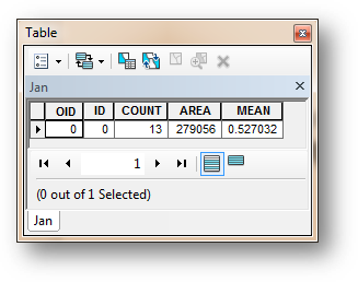
The mean NDVI value for the month of January within the AOI extent is 0.53.
Compute the Zonal Statistics for the remaining 11 months. Name the outputs Feb.dbf, Mar.dbf, etc…
When complete, you should see 12 NDVI tables in your TOC.
Next, you will combine the tables into a single table.
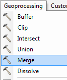
From the Geoprocessing pull-down menu, select Merge.
In the Merge window, add all twelve tables. Make sure that the tables appear in chronological order!
Save the output table in the NDVI folder and name it all_NDVI.dbf (don’t forget to specify the .dbf extension)
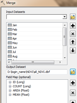
Click OK to run the geoprocess.
The new all_NDVI table will be added to the TOC.
In the last and final step, you will graph the results.
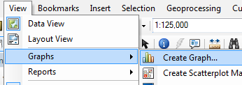
From the View pull-down menu, go to Graphs and select Create Graph.
In the Create Graph Wizard window, select Vertical Line as graph type.
Select all_NDVI as the table.
Select MEAN for the Y field.
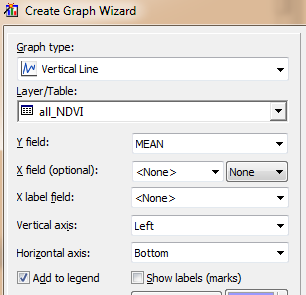
Click Next.
Click Finish.
The output order follows the month order in the all_NDVI table (which explains why their order in the Merge function was critical).
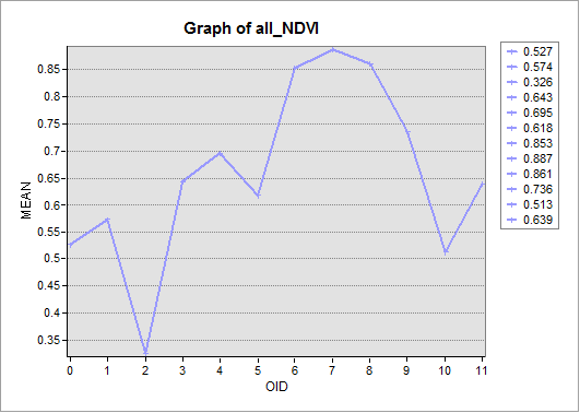
Note the peak NDVI values in Summer--as expected. You will also note that the NDVI values for the winter months are not low. This is because most trees in the AOI are evergreens (hence, they remain green year round).
Save your Map document.
Close your map document
This concludes this session.
![]() Manuel Gimond, last modified on 3/2/2012
Manuel Gimond, last modified on 3/2/2012