Creating and mosaicking NDVI rasters for Colby wooded areas
|
1. Create a folder called NDVI_colby. On DIA 322 computers, you might want to create this folder in your user Documents folder (e.g. C:\Users\jdoe\Documents\NDVI_colby). On the DIA 222 computers, you might want to create this folder on the D: drive under D:\course number\user name\ (e.g. D:\ES212\jdoe\NDVI_colby). 2. Under your login_name folder, create another folder called NDVI_colby. 3. Download the data for this exercise and extract the contents of the NDVI.zip file to your newly created NDVI directory on the D: drive. |
Step 1: Viewing a multi-band image
Step 2: Creating an NDVI Raster
Step 3: Mosaicing Raster Layers
Step 4: Managing Raster File Size
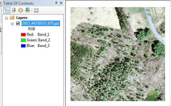
Load one of the CIR images into a blank ArcMap document.
Note: The data were downloaded from MEGIS’ Orthoimagery viewer.
By default, ArcMap will load the first three bands of the image file and assign these bands to the screen’s red, green and blue colors. These CIR images have the following band configurations. Note: the band order does not match the wavelength order (i.e. the blue wavelength is swapped with the red wavelength):
|
Band number |
Associated wavelength |
|
1 |
Red (600 – 700 nm) |
|
2 |
Green (500 – 600 nm) |
|
3 |
Blue (400 – 500 nm) |
|
4 |
Near Infrared ( >700 nm) |
The addition of a near-infrared (NIR) band provides us with a unique
perspective of land surface features. We can add this band to our display by
assigning it to the digital screen’s Red gun and bumping the red band and green
band down the color gun ladder. This implies that the blue band will no longer
be displayed.
Open the image layer’s properties window and select Symbology.
Next, assign band_4, band_1 and band_2 to the Red, Green and Blue display color guns.
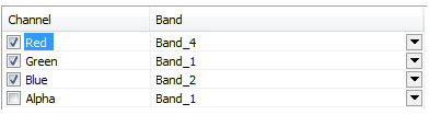
Click OK to close the Properties window.
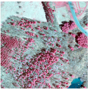
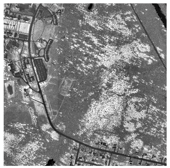
The above band combination generates a view called a false color composite.
|
|
Note the prominence of the evergreens in this scene. They appear as red features. Why is this? How does the spectral shape of plant reflectance explain this? |
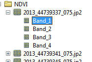
Next you will load the NIR and Red bands as individual layers.
This is done by double-clicking on the *.jp2 raster layer then loading the band_1 and band_4 layers separately.
Next, you will compute the NDVI values for each pixel in the scene using the two bands.
Open the raster calculator (under Spatial Analyst >> Map Algebra).
The NDVI is computed as (NIR - Red) / (Red + NIR). However, because the rasters in this exercise are stored as integers, ArcMap will assume that the output must be stored as integers as well. It therefore follows that any value in the output raster will be rounded to the nearest integer—this is not what we want since NDVI values can take on any values between -1 and 1. We will therefore need to wrap the numerator with the Float() function. This function will force ArcMap to treat the pixel values as floats and not integers.
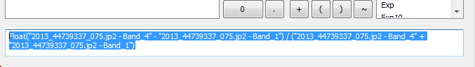
Create the following expression in the expression box. It might be easier to double-click on the layer names to carry them over into the expression box instead of typing them in directly.
Float("2013_44739337_075.jp2 - Band_4" - "2013_44739337_075.jp2 - Band_1") / ("2013_44739337_075.jp2 - Band_4" + "2013_44739337_075.jp2 - Band_1")
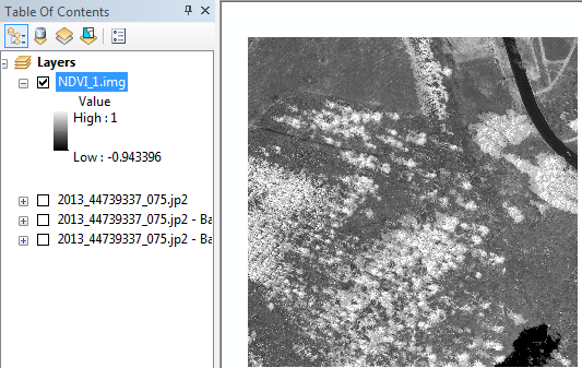
You will name the output NDVI_1.img.
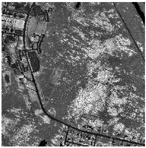
The output is a single band raster that maps NDVI values for each pixel.
|
|
Can you interpret the map? What does a high NDVI value indicate? How about a low NDVI value? |
Next, generate NDVI rasters from the other eight .jp2 raster files.
The nine rasters produce a tiled layout of a section of the Colby campus.
Next, you will mosaic the nine NDVI rasters into a single raster. To “mosaic” (merge) vector layers, we can use the Merge geoprocess tool. For raster layers, another mosaic tool must be used: the Mosaic to New Raster tool (under Data Management Tools >> Raster >> Raster Dataset).
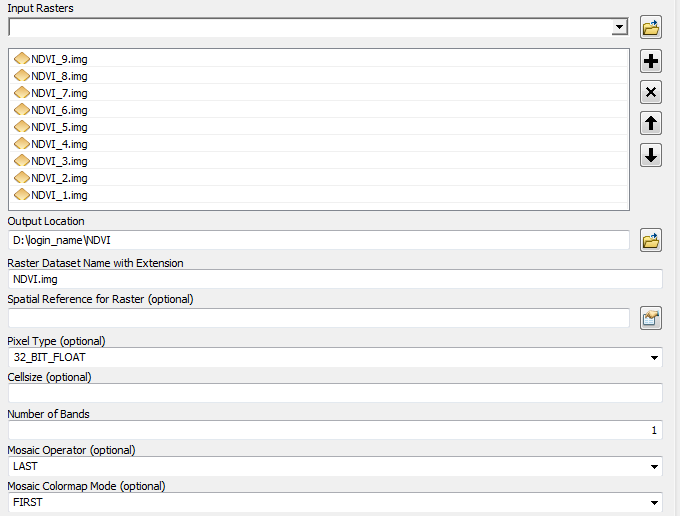
Using the Mosaic to New Raster tool, mosaic all nine raster layers to create a new raster: NDVI.img. Make sure to select the 32_bit_float option (since the data are stored as floats and not integers) and set the output number of bands to 1 (the NDVI layers are made up of a single band only).
The output raster is a single mosaic of all nine rasters.
A downside to storing a raster data as a Float is the large disk space it can consume. The mosaicked NDVI raster file takes up more than 850 MB of disk space. This is unnecessary. A common workaround is to scale the pixel values before storing the file as an integer.
Using the raster calculator, multiply all pixel values by 1000 and force the output value as an integer using the following expression:
Int(“NDVI.img” * 1000)
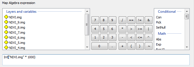
Name the output NDVI_1000.img.
ArcGIS may output a 32-bit integer raster. This reduces the file size a little bit, but we can do better (we don’t need 32-bit of storage for a small range of values). We will therefore copy the raster to a new 16-bit signed raster (which can handle values that range from -32,768 to 32,767).
Open the Copy Raster tool (Data Management >> Raster >> Raster Dataset) and fill out the parameters as specified below (your output raster file location may differ).
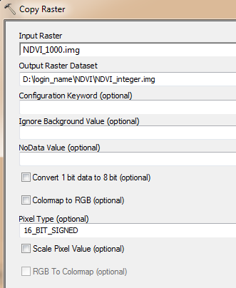
Click OK to run the geoprocess.
Your output file size should now be around 400 MB (about half of its original size).
Thought exercise: Could you have saved the raster as a signed 8 bit raster instead of a 16 bit raster? If so, how would you have scaled (transformed) the NDVI values (i.e. what range of NDVI values would the signed 8 bit raster take on)?
![]() Manuel Gimond, last modified on 1/30/2015
Manuel Gimond, last modified on 1/30/2015