Viewshed analysis
|
· Create a folder called Viewshed somewhere under your personal directory (e.g. C:\Users\jdoe\Documents\Tutorials\Viewshed\). · Download the data for this exercise then extract the contents of Viewshed.zip into your newly created Viewshed directory. |
In this exercise, you will learn to generate viewsheds for given point locations using an elevation raster. This tutorial requires that you enable the Spatial Analyst extension under Customize >> Extensions.
Step 2: Defining the observer offset from the ground
Step 3: Creating the viewshed raster
Open the Viewshed.mxd document.
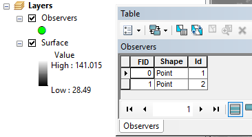
The map document consists of two layers: a Lidar derived raster surface model of the Colby campus and two point locations for which a viewshed is to be computed.
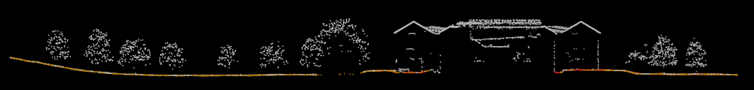
The surface raster does not represent ground elevation but includes both exposed ground and none ground surfaces such as trees and buildings. A profile view of the original Lidar data may look something like this:
The raster’s profile of this sample Lidar cross section looks like,
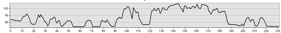
where the x and y unites are in meters.
Unlike the ground elevation raster, the surface elevation raster includes obstructions such as trees and buildings which is a more realistic representation of the viewshed. The original Lidar point data file was downloaded from USGS’ National Map website.
By default, ArcMap’s Viewshed tool will compute the viewshed relative to the observer’s raster surface elevation value. This may not be realistic since the observer’s eye level may be several feet above the ground surface. You may also want to apply an offset if the observer point location happens to coincide with a non-ground elevation associated with a tree for example (in which case you would apply a negative offset). You can define the observer’s height above (or below) the raster elevation value by adding a new attribute, OFFSETA, to the point layer’s attribute table.
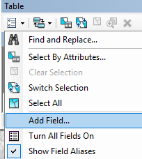
Right-click on the Observers layer in the TOC then select Open Attribute Table.
Click on the Table Options icon ![]() in the upper left-hand
corner of the Attribute table and select Add Field.
in the upper left-hand
corner of the Attribute table and select Add Field.
Create a new field called OFFSETA. Make it a float data type.
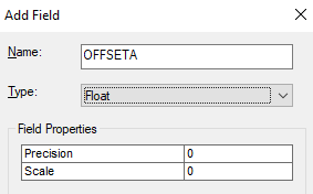
Click OK to close the Add Field window and accept the change.
Next, we’ll enter an edit session to modify the OFFSETA values.
Right-click on the Observers layer and select Edit Features >> Start Editing.
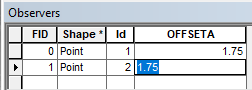
Now that we are in an edit session, we can enter the height offset values in the Observer’s attribute table. The entered height units are in the same elevation units defined by the surface raster (meters in our example). We will therefore enter offset units of 1.75 meters (the average human height).
Enter 1.75 in both OFFSETA rows.
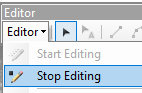
In the Editor Tool bar, select Save Edits.
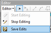
In the same Editor Tool bar, select Stop Editing.
Note that other observer parameters can be defined in the attribute table. The following lists the attribute values and a brief description of their use.
|
SPOT |
The observer’s elevation (following the same vertical datum defining the surface raster). This differs from OFFSETA in that the observer’s height is explicitly defined above some reference height (usually set to mean sea level). |
|
AZIMUTH1, AZIMUTH2 |
If the viewing direction is to be limited to a certain direction, you can use these attributes to define the starting and ending azimuthal angles. The angular units are in degrees and are measured clockwise with 0° pointing north. |
|
VERT1, VERT2 |
If the viewing direction is to be limited to an elevation, you can use these attributes to define the starting an ending vertical angles. The angular measurement is in degrees and ranges from -90° (pointing straight down) to 90° (pointing straight north). |
|
RADIUS1, RADIUS2 |
You can limit the starting and ending depth of your view extent. For example, if you want to restrict the viewshed to a distance no shorter than 100 meters and no longer than 400 meters, set RADIUS1 equal to 100 and RADIUS2 to 400 (this assumes that the map units are also in meters). |
In the ArcToolbox ![]() , open Spatial Analyst Tools
>> Surface >> Viewshed.
, open Spatial Analyst Tools
>> Surface >> Viewshed.
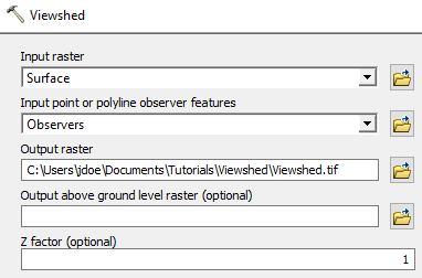
Click OK to run the geoprocess.
Note that if your viewshed radius covers a large enough distance where earth curvature is a factor, check off the Use earth curvature checkbox.
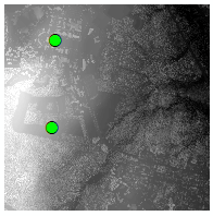
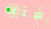
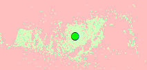
The output is a binary raster where a pixel value of 1 (symbolized in green) highlights locations that can be seen from the observation points.
The output can also be viewed in 3D Scene.
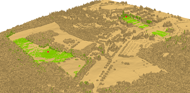
Note that the viewshed output does not distinguish between observation points. If distinct viewsheds are to be identified for each observation, then the Viewshed tool needs to be run separately for each point feature.
© Manny Gimond, 6/5/2018