PPM: Exploring 1^st order effects

Author

Manny Gimond

Data for this tutorial can be downloaded from here. Don’t forget to unzip the files to a dedicated folder on your computer.

Don’t forget to set the R session to the project folder via Session >> Set Working Directory >> Choose Directory.

Loading the data into R

First, we’ll load the point pattern dataset, then we’ll load two different raster datasets that will represent two separate 1^st order effects we suspect may help explain the distribution of stores within the study extent.

# Load packages
library(spatstat)
library(sf)
library(terra)

# Read state polygon data
s    <- st_read("MA.shp")
w    <- as.owin(s)
w.km <- rescale.owin(w, 1000)

# Read Walmart point data
s    <- st_read("Walmarts.shp")
p    <- as.ppp(s)
p.km <- rescale.ppp(p, 1000)
marks(p.km)  <- NULL
Window(p.km) <- w.km

# Read population density raster
img     <- rast("pop_sqmile.tif")
df      <- as.data.frame(img, xy = TRUE)
pop     <- as.im(df)
pop.km  <- rescale.im(pop, 1000)

# Read median income raster
img      <- rast("median_income.tif")
df       <- as.data.frame(img, xy = TRUE)
inc      <- as.im(df)
inc.km   <- rescale.im(inc, 1000)

Note that later in the script, we will make use of the effectfun() that requires that the raster layer be stored as a double data type. You can tell if your raster is stored as a double by typing typeof(inc.km[]), for example. If it’s not stored as a double, you can force it to a double using the as.double() function (e.g. inc[] <- as.double(inc[])).

Let’s plot each raster with the Walmart point overlay. We’ll use R’s base plotting environment.

plot(pop.km, ribside="bottom", main="Population")
plot(p.km, pch = 20, col=rgb(1,1,1,0.5), add=TRUE)

plot(inc.km, ribside="bottom", main="Income")
plot(p.km, pch = 20, col=rgb(1,1,1,0.6), add=TRUE)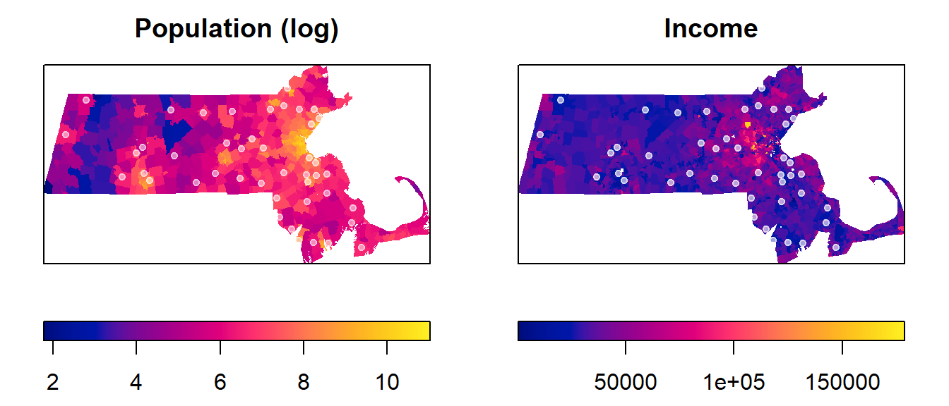

Modeling the Covariate Effect

We will first develop two different models that we think might define the Walmart’s point intensity. Recall that intensity is a property of the underlying “process” (one being defined by the distribution of population density and the other being defined by the distribution of income)–this differs from density which is associated with the observed pattern. These models are represented in our R script by two raster layers: a population raster and an income raster. These models will be alternate models that we’ll denote as Mpop and Minc in the script. The models’ structure will follow the form of a logistics model, but note that the models can take on many different forms and different levels of complexity.

We’ll also create the null model, Mo, which will assume a spatially uniform (homogeneous) covariate. In other words, Mo will define the model where the intensity of the process is assumed to be the same across the entire study extent.

Mpop <- ppm(p.km ~ pop.km) # Population model

Warning: Values of the covariate 'pop.km' were NA or undefined at 3.4% (17 out
of 504) of the quadrature points. Occurred while executing: ppm.ppp(Q = p.km,
trend = ~pop.km, data = NULL, interaction = NULL)

Minc <- ppm(p.km ~ inc.km) # Income model

Warning: Values of the covariate 'inc.km' were NA or undefined at 3.2% (16 out
of 504) of the quadrature points. Occurred while executing: ppm.ppp(Q = p.km,
trend = ~inc.km, data = NULL, interaction = NULL)

Mo   <- ppm(p.km ~ 1)      # Null model

Let’s explore the model parameters. First, we’ll look at Mpop.

Mpop

Nonstationary Poisson process
Fitted to point pattern dataset 'p.km'

Log intensity:  ~pop.km

Fitted trend coefficients:
  (Intercept)        pop.km 
-6.2705211696  0.0001136109 

                 Estimate         S.E.       CI95.lo       CI95.hi Ztest
(Intercept) -6.2705211696 1.640539e-01 -6.592061e+00 -5.9489813892   ***
pop.km       0.0001136109 4.366087e-05  2.803713e-05  0.0001991846    **
                  Zval
(Intercept) -38.222318
pop.km        2.602121
Problem:
 Values of the covariate 'pop.km' were NA or undefined at 3.4% (17 out of 504) 
of the quadrature points

The values of interest are the intercept (whose value is around -6.3) and the coefficient pop.km (whose value is around 0.0001). Using these values, we can construct the mathematical relationship (noting that we are using the population raster and not the original population raster values):

\[ Walmart\ intensity(i)= e^{−6.3 + 0.0001\ population\ density_i} \] The above equation can be interpreted as follows: if the population density is 0, then the Walmart intensity is \(e^{−6.3}\) which is very close to 0. So for every unit increase of the population density (i.e. one person per square mile), there is an increase in Walmart intensity by a factor of \(e^{0.0001}\) stores per square kilometer.

Likewise, we can extract the parameters from the Minc model and construct its equation.

Minc

Nonstationary Poisson process
Fitted to point pattern dataset 'p.km'

Log intensity:  ~inc.km

Fitted trend coefficients:
  (Intercept)        inc.km 
-5.576942e+00 -1.654792e-05 

                 Estimate         S.E.       CI95.lo       CI95.hi Ztest
(Intercept) -5.576942e+00 5.258426e-01 -6.607574e+00 -4.546309e+00   ***
inc.km      -1.654792e-05 1.490546e-05 -4.576209e-05  1.266624e-05      
                  Zval
(Intercept) -10.605725
inc.km       -1.110192
Problem:
 Values of the covariate 'inc.km' were NA or undefined at 3.2% (16 out of 504) 
of the quadrature points

\[ Walmart\ intensity(i) = e^{−5.58\ −1.66e^{−5}\ Income(i)} \] Note the negative (decreasing) relationship between income distribution and Walmart density.

Next, we’ll extract the null model results:

Mo

Stationary Poisson process
Fitted to point pattern dataset 'p.km'
Intensity: 0.002086305
             Estimate      S.E.   CI95.lo   CI95.hi Ztest      Zval
log(lambda) -6.172361 0.1507557 -6.467836 -5.876885   *** -40.94281

This gives us the following equation for the homogeneous process:

\[ Walmart\ intensity(i) = e^{−6.17} = 0.00209 \]

which is nothing more than the number of stores per unit area (44 stores / 21,000km² = 0.00209).

Plotting the competing models

OP <- par(mfrow = c(1,2), mar = c(4,4,2,1))  # This creates a two-pane plotting window

plot(effectfun(Mpop, "pop.km", se.fit = TRUE), main = "Population",
     ylab = "Walmarts per km2", xlab = "Population density", legend = FALSE)

plot(effectfun(Minc, "inc.km", se.fit = TRUE), main = "Income",
     ylab = "Walmarts per km2", xlab = "Income", legend = FALSE)

par(OP) # This reverts our plot window back to a one-panel window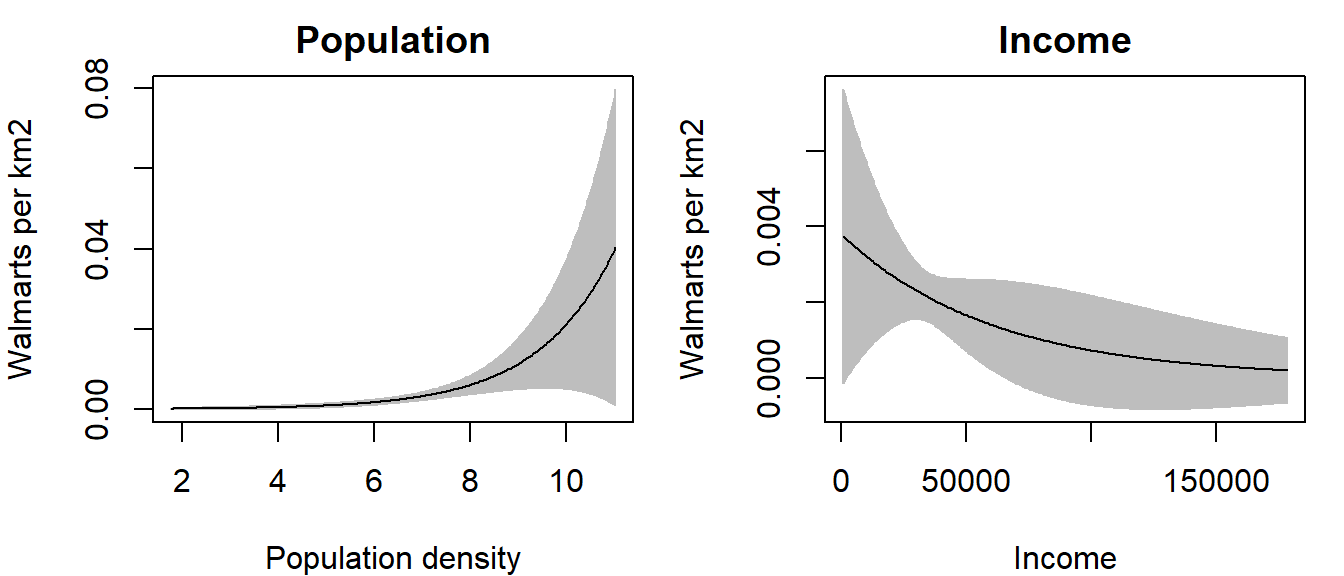

Note the difference in relationships between the two models. In the first plot, we note a slightly increasing relationship between Walmart intensity and population density; this is to be expected since you would not expect to see Walmart stores in underpopulated areas. In the second plot, we note an inverse relationship between Walmart intensity and income—i.e. as an area’s income increases, the Walmart intensity decreases.

The grey envelopes encompass the 95% confidence interval; i.e. the true estimate (black line) can fall anywhere within this envelope. Note how the envelope broadens near the upper end of the population density values–this suggests wide uncertainty in the estimated model.

To assess how well the above models explain the relationship between covariate and Walmart intensity, we will turn to hypothesis testing.

Testing the Covariate Effect

To formally assess whether the covariate-based model provides a significantly better fit than the null model, we need a way to reduce that comparison to a single number. That number is called the likelihood‑ratio test (LRT) statistic.

A model that fits the data better gives a higher likelihood for the observed pattern.
The LRT statistic measures how much better the more complex model Mpop or Minc fit the data than the simpler “null” model Mo.

Think of the LRT as a kind of “distance” between the two models’ explanations of the same point pattern.

Small LRT statistic -> the alternative model explains the pattern almost equally well
Large LRT statictic -> the alternative model explains the pattern noticeably better

The `Mpop` model test

We’ll first apply a LRT test for the Mpop model.

anova(Mo, Mpop, test = "LRT") # Compare null to population model

Warning: Values of the covariate 'pop.km' were NA or undefined at 3.4% (17 out
of 504) of the quadrature points. Occurred while executing: ppm.ppp(Q = p.km,
trend = ~pop.km, data = NULL, interaction = NULL,

Warning: Models were re-fitted after discarding quadrature points that were
illegal under some of the models

Analysis of Deviance Table

Model 1: ~1      Poisson
Model 2: ~pop.km     Poisson
  Npar Df Deviance Pr(>Chi)  
1   18                       
2   19  1   4.2968  0.03819 *
---
Signif. codes:  0 '***' 0.001 '**' 0.01 '*' 0.05 '.' 0.1 ' ' 1

In spatstat, the LRT statistic appears as the difference in deviance in the output. We compare this value to a reference distribution–a picture of how big the LRT statistic (i.e. the difference-in-deviance value in the output) would usually be if the null model really were adequate. The following figure shows this distribution with the observed statistic displayed as a veritcial blue line.

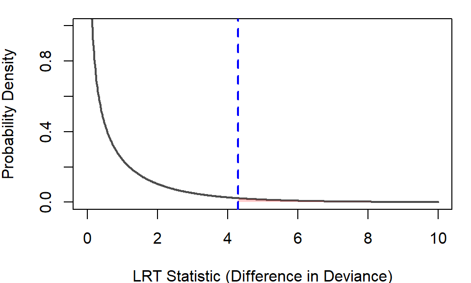
The reference distribution addresses the question “If the null model were true, how likely is it that random noise alone would produce an LRT statistic (difference-in-deviance) this large (4.2968) or larger?. The probability can be extracted from the plot or from the anova() output under the pr heading–this is the p-value. For the Mpop model, the p-value is 0.03819 or 3.8%.

This means that if the population density had no real effect, then a statistic as large as 4.2968 would occur only about 3.8% of the time. Because this is fairly unlikely, we interpret the result as evidence that including population density does help explain where points occur.

The `Minc` model test

anova(Mo, Minc, test = "LRT") # Compare null to income model

Warning: Values of the covariate 'inc.km' were NA or undefined at 3.2% (16 out
of 504) of the quadrature points. Occurred while executing: ppm.ppp(Q = p.km,
trend = ~inc.km, data = NULL, interaction = NULL,

Warning: Models were re-fitted after discarding quadrature points that were
illegal under some of the models

Analysis of Deviance Table

Model 1: ~1      Poisson
Model 2: ~inc.km     Poisson
  Npar Df Deviance Pr(>Chi)
1   17                     
2   18  1   1.3388   0.2473

The model using median income (Minc) shows a very different result. The LRT statistic for Minc is 1.3388, yielding a p‑value of 0.2473–roughly 25%. This value is well within the range of what we would expect just by chance if the null model (constant intensity) were true. A statistic this small is not unusual under the null model, meaning that including income as a covariate does not provide strong evidence of improvement. From this, we can conclude that income does not significantly explain the observed point distribution, at least not in the way population density does. Together, these results suggest that population density is a more relevant predictor of point intensity than income in this dataset.

Additional Guidance on Interpreting p‑values

Finally, it’s important not to treat the 0.05 cutoff as a strict “significant / not significant” decision rule. The value 0.05 has no theoretical justification, it is simply a historical convention—and relying on it too rigidly can lead to oversimplified or misleading interpretations. Instead, interpret the p‑value as a continuous measure of how surprising your data would be if the null model were true. A smaller p‑value means the observed improvement is less likely to be due to chance alone, while a larger p‑value means the improvement is more consistent with random variation. This perspective helps you think in terms of evidence and uncertainty, rather than treating statistical testing as a binary yes/no decision.