| ggplot2 |
|---|
| 4.0.2 |
27 Non-parametric Bivariate Modeling with Loess
In the previous chapter, we explored parametric models such as linear and polynomial regression. These models require specifying a functional form—like a straight line or a quadratic curve-before fitting the data. While parametric models are powerful and interpretable, they can be limiting when the true relationship between variables is complex or unknown.
Non-parametric models offer a flexible alternative. They do not assume a specific functional form and instead allow the data to guide the shape of the model. One such method is loess (locally weighted regression), which fits simple models to localized subsets of the data to build a smooth curve.
In this chapter, we will explore how loess works and how it is constructed.
27.1 Non-parametric fit
Polynomial models used to fit lines to data are classified as parametric models. These models require defining a specific functional form (e.g., linear, quadratic) a priori, which is then fitted to the data. By imposing this predefined structure, parametric models make strong assumptions about the underlying relationship between variables.
In contrast, non-parametric models belong to a class of fitting strategies that do not assume a specific structure for the data. Instead, these models are designed to adapt flexibly, allowing the data to reveal its inherent patterns and relationships. One such method used in this course is the loess fit, a locally weighted regression approach.
27.2 Loess
A flexible curve-fitting method is the loess curve (short for local regression, also known as local weighted regression). This technique fits small segments of a regression line across the range of x-values and links the midpoints of these segments to generate a smooth curve. The range of x-values contributing to each localized regression lines is controlled by the span parameter, \(\alpha\), which typically ranges from 0.2 to 1 (though it can exceed 1 for smaller datasets). Another key parameter, \(\lambda\), specifies the polynomial order of the localized regression lines and is typically 1 or 2.
27.3 How a loess is constructed
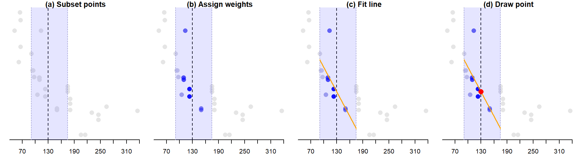
Behind the scenes, each point (\(x_i\), \(y_i\)) that defines the loess curve is constructed as follows:
A subset of data points closest to point \(x_i\) are identified (\(x_{130}\) is used as an example in the figure below). The number of points in the subset is identified by multiplying the bandwidth \(\alpha\) by the total number of observations. In the
mtcars’mpgvs.hpdataset, \(\alpha\) is set to 0.5. The number of points defining the subset is thus 0.5 * 32 = 16. The region encompassing these points is displayed in a light blue color.The points in the subset are assigned weights. Greater weight is assigned to points closest to \(x_i\). The weights define the points’ influence on the fitted line. Different weighting techniques can be implemented in a loess with the
gaussianweight being the most common. Another weighting strategy we will also explore later in this course is thesymmetricweight.A regression line is fit to the subset of points. Points with smaller weights will have less leverage on the fitted line than points with larger weights. The fitted line can be either a first order polynomial fit or a second order polynomial fit.
Next, the value \(y_i\) from the regression line is computed (red point in panel (d)). This is one of the points that will define the shape of the loess.
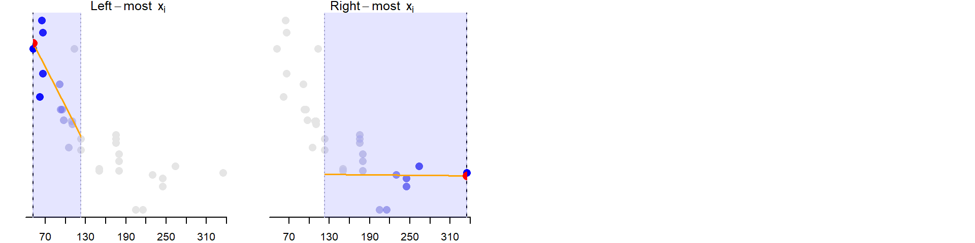
The above steps are repeated for as many \(x_i\) values practically possible. Note that when \(x_i\) approaches an upper or lower limit, the subset of points is no longer centered on \(x_i\). For example, when estimating \(x_{52}\), the sixteen closest points to the right of \(x_{52}\) are selected. Likewise, for the upper bound \(x_{335}\), the sixteen closest points to the left of \(x_{335}\) are selected.
In the following example, just under 30 loess points are computed at equal intervals. This defines the shape of the loess.
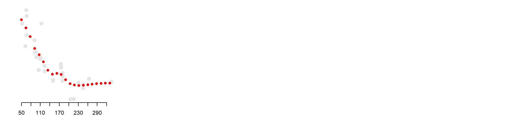
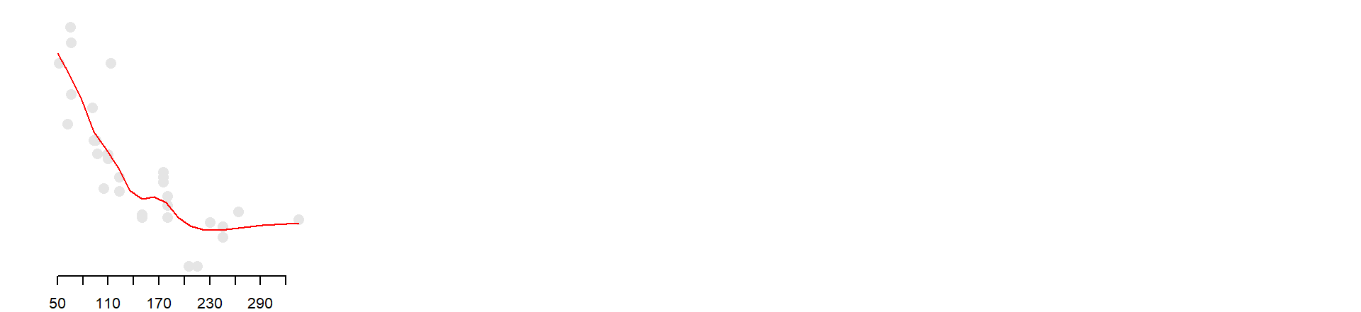
It’s more conventional to plot the line segments than it is to plot the points.
27.4 Span sensitivity
The span parameter in a loess model controls the width of the neighborhood used to fit each local regression. Smaller span values result in more localized fits, which can capture fine-grained patterns but may also lead to overfitting. Larger span values produce smoother curves by averaging over broader neighborhoods, which can help reveal general trends but may miss subtle local features.
Below is a comparison of loess fits applied to the mtcars dataset (miles-per-gallon vs. horsepower) using four different span values and a polynomial degree of 1:
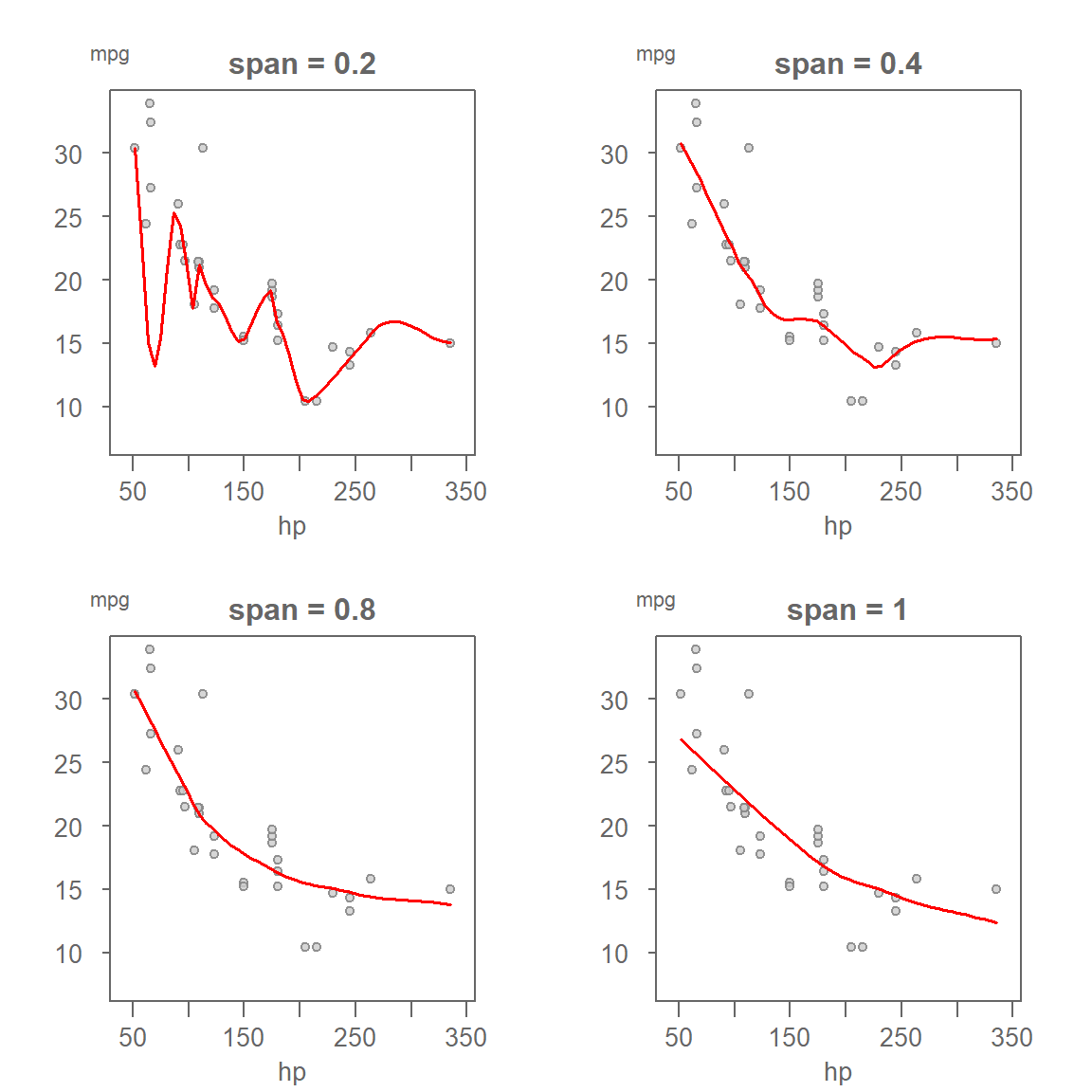
- Span = 0.2: The curve closely follows the data points, capturing small fluctuations. This can be useful for detecting local structure but risks overfitting noise.
- Span = 0.4: A balanced fit that captures the overall trend while still being responsive to local changes.
- Span = 0.8 and 1.0: These produce smoother curves that emphasize the broader trend, potentially overlooking finer details.
Avoiding overfitting
Using a very small span (e.g., < 0.3) can lead to a curve that reacts to random variation rather than meaningful structure. This is especially problematic with small datasets or noisy measurements. To avoid overfitting:
- Start with a moderate span (e.g., 0.5) and adjust based on visual inspection.
- Use residual plots to check whether the loess fit removes structure effectively.
- Consider the goal of the analysis: if you’re exploring broad trends, a larger span may be more appropriate.
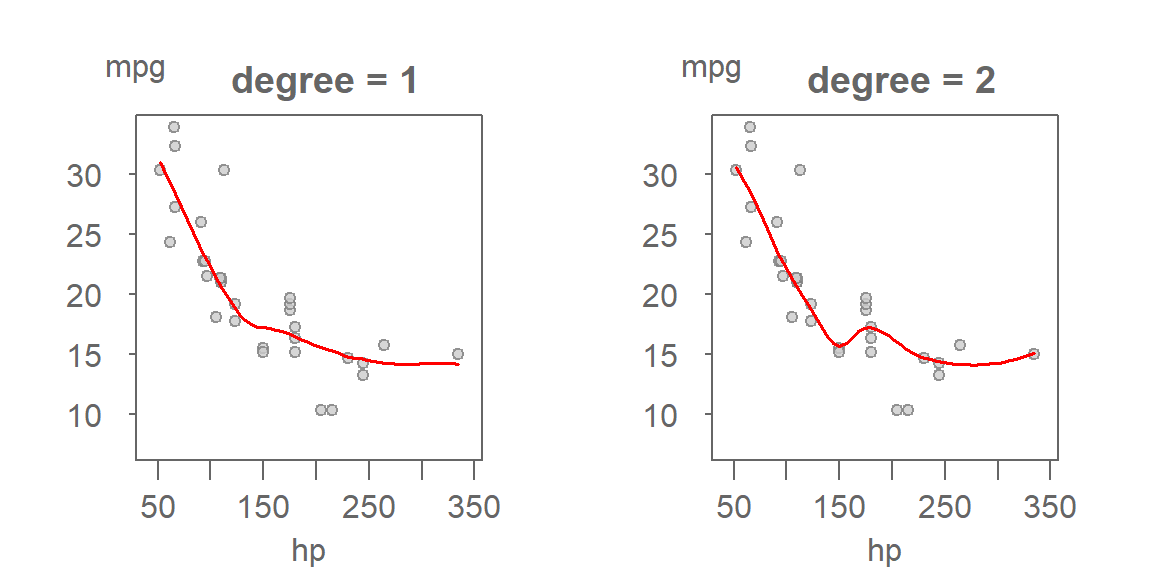
27.5 Polynomial degree in loess
In addition to the span parameter, loess models also allow you to specify the degree of the local polynomial used to fit each neighborhood. The two most common choices are:
- Degree = 1: Fits a local linear regression to each neighborhood.
- Degree = 2: Fits a local quadratic regression, allowing for curvature within each neighborhood.
When to Use Degree 1 A first-order polynomial (linear) is often sufficient when the underlying relationship is smooth and monotonic. It tends to be more stable and less sensitive to noise, especially when combined with a small span.
When to Use Degree 2 A second-order polynomial (quadratic) can capture local curvature, making it useful when the data shows bends or inflection points. However, it is more sensitive to outliers and can introduce wiggles in the fitted curve if the span is too small. This is the default choice in many R loess implementations.
Practical Tip If you’re using a small span, it’s generally safer to stick with degree = 1 to avoid overfitting. If you’re using a larger span, degree = 2 may help reveal subtle curvature without introducing instability.
27.6 Choosing between polynomial and loess Models
While loess offers a flexible data-driven approach to modeling, there are still good reasons to consider parametric polynomial models in certain situations.
27.6.1 When to Use a Polynomial Model
- Interpretability: Polynomial models provide explicit equations that are easy to interpret and communicate.
- Simplicity: A low-order polynomial (e.g., linear or quadratic) may be sufficient to capture the main trend in the data.
- Statistical inference: If your goal is to test hypotheses (e.g., is the slope significantly different from zero?), parametric models are more appropriate.
27.6.2 When to use loess
- Exploration: Loess is ideal for uncovering structure in the data without assuming a specific form.
- Nonlinearity: When the relationship between variables is complex or unknown, loess can adapt to local patterns.
- Visualization: Loess provides smooth, intuitive curves that help reveal trends in scatter plots.
In practice, loess is often used during the exploratory phase to guide model selection, while polynomial models may be used for confirmatory analysis or reporting.
27.7 Generating a loess model in base R
The loess fit can be computed in R using the loess() function. It takes as arguments span (\(\alpha\)), and degree (\(\lambda\)).
# Fit loess function
lo <- loess(mpg ~ hp, mtcars, span = 0.5, degree = 1)

# Predict loess values for a range of x-values
lo.x <- seq(min(mtcars$hp), max(mtcars$hp), length.out = 50)
lo.y <- predict(lo, lo.x)
The modeled loess curve can be added to the scatter plot using the lines function.
plot(mpg ~ hp, mtcars)
lines(lo.x, lo.y, col = "red")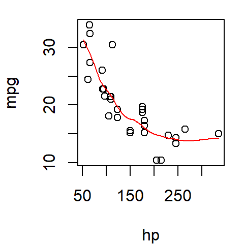
27.8 Generating a loess model in ggplot
In ggplot2 simply pass the method="loess" parameter to the stat_smooth function.
library(ggplot2)

ggplot(mtcars, aes(x = hp, y = mpg)) + geom_point() +
             stat_smooth(method = "loess", se = FALSE, span = 0.5)
ggplot defaults to a second degree loess (i.e. the small regression line elements that define the loess are modeled using a 2nd order polynomial and not a 1st order polynomial). If a first order polynomial is desired, you need to include an argument list in the form of method.args=list(degree=1) to the stat_smooth function.
library(ggplot2)

ggplot(mtcars, aes(x = hp, y = mpg)) + geom_point() +
             stat_smooth(method = "loess", se = FALSE, span = 0.5,
                         method.args = list(degree = 1) )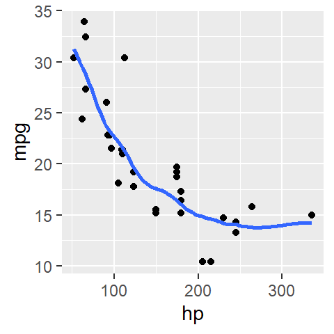
27.9 Summary
Loess offers a flexible, non-parametric approach to modeling bivariate relationships without assuming a fixed functional form. By fitting localized regressions across the range of the independent variable, loess can reveal subtle patterns and trends that parametric models might miss. Two key parameters—span and degree—control the behavior of the fit:
- Span determines the width of the neighborhood used for each local fit. Smaller spans capture fine detail but risk overfitting, while larger spans smooth out noise and emphasize broader trends.
- Degree defines the polynomial order of the local regression. A linear fit (degree = 1) is more stable and less sensitive to outliers, while a quadratic fit (degree = 2) can capture curvature but may introduce instability if the span is too small.
Understanding how these parameters influence the loess curve is essential for balancing flexibility with interpretability. Loess is especially useful in exploratory data analysis, where the goal is to uncover structure rather than impose it.