3-point summary plot — eda

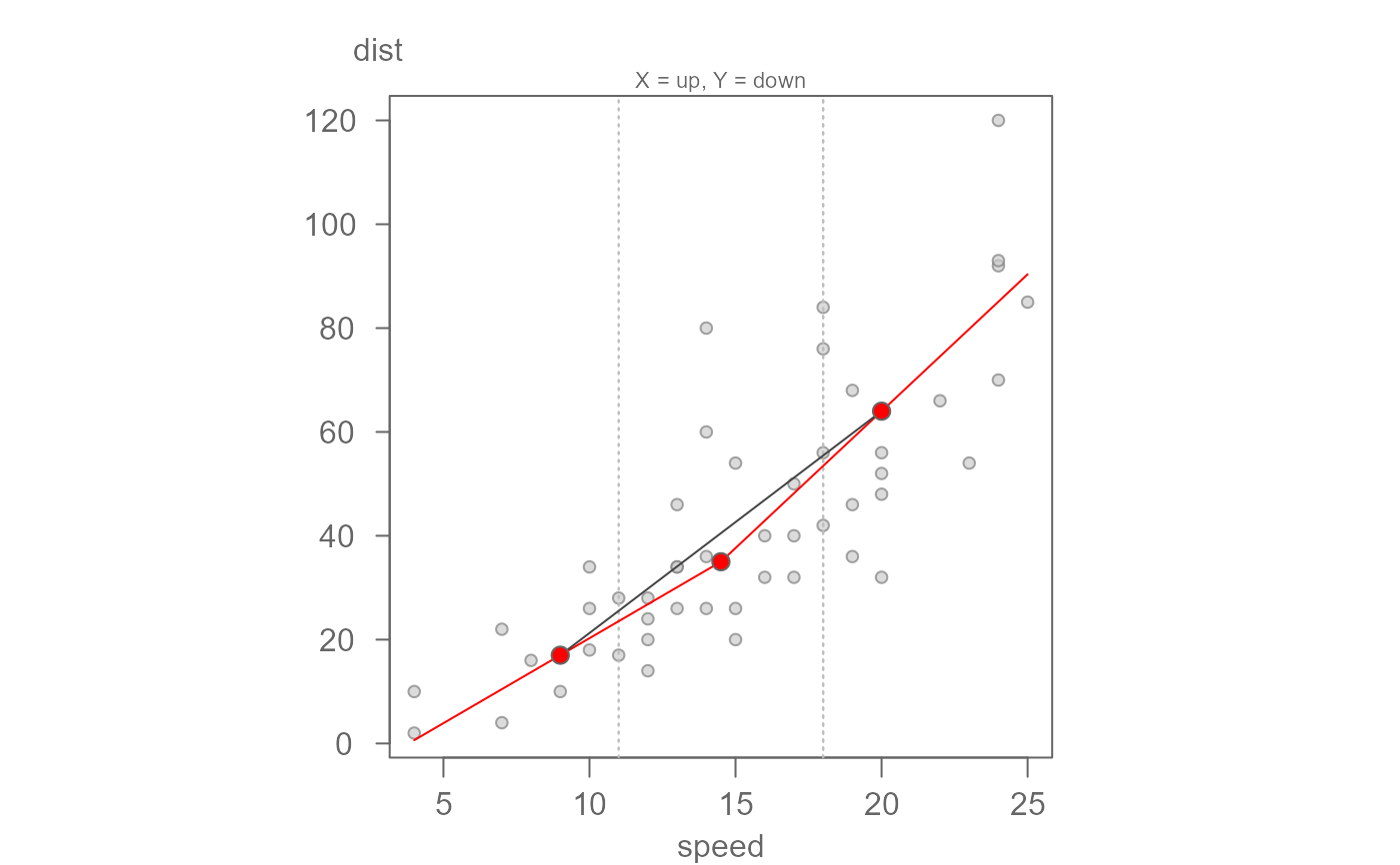
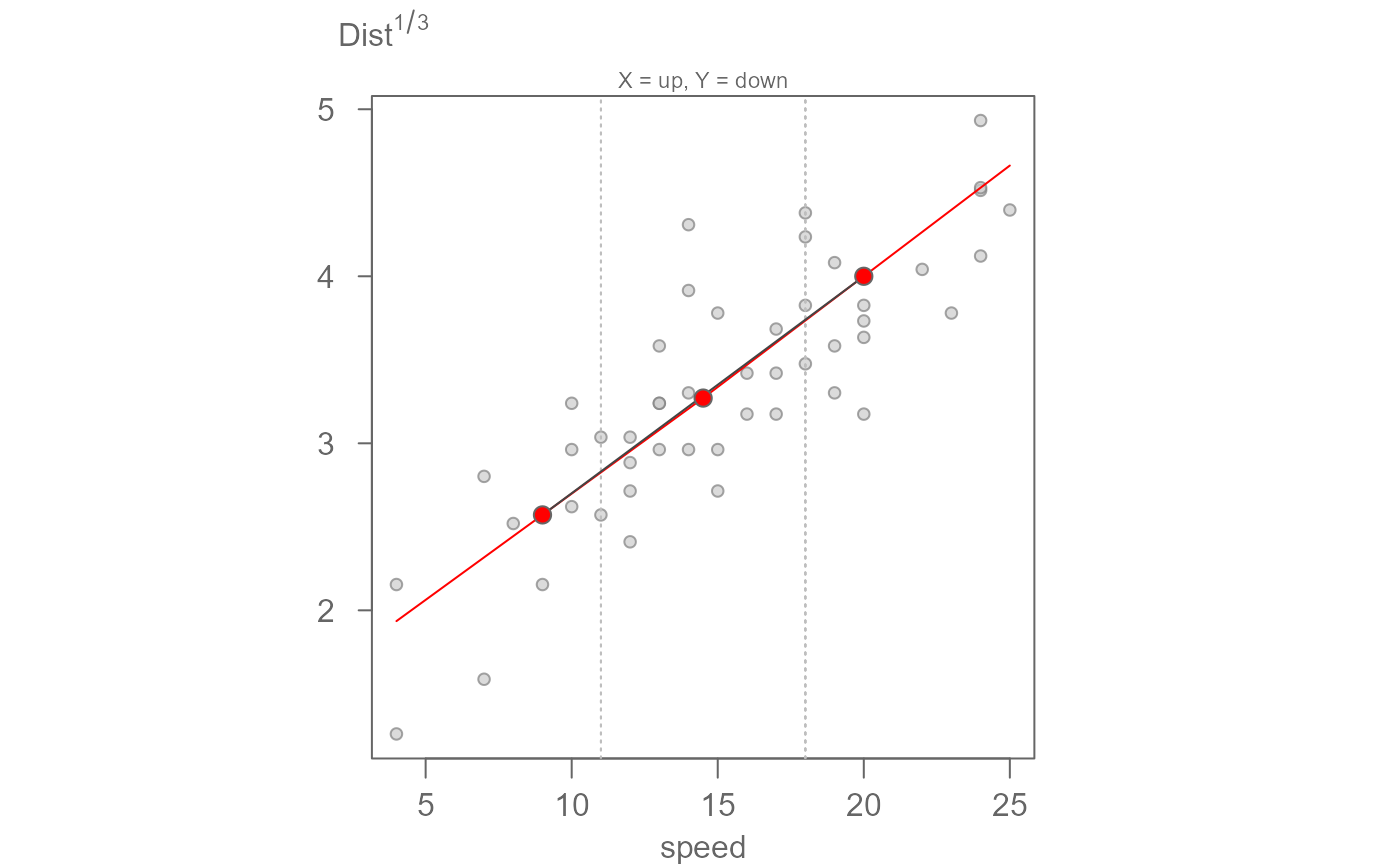
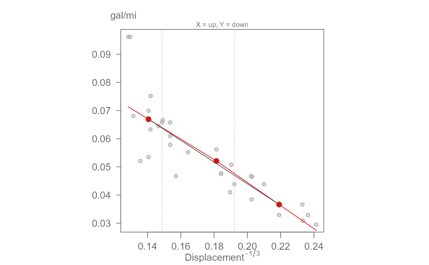
eda_3pt splits the data into 3 groups (whose summary locations are defined by their respective medians), and two half slopes linking the groups. The function will return a scatter plot showing the half-slopes in red solid lines. The solid grey slope linking both tail-end groups shows the desired shape for both half-slopes. The goal is to have the two halve slopes line up as closely as possible to the solid grey slope via re-expression techniques when seeking a linear relationship between both variables.

The function will also return the half-slopes ratio hsrtio and the direction of re-expression for both X and Y values on the ladder of powers.

Usage

eda_3pt(
  dat,
  x,
  y,
  px = 1,
  py = 1,
  tukey = TRUE,
  axes = TRUE,
  pch = 21,
  equal = TRUE,
  p.col = "grey50",
  p.fill = "grey80",
  size = 0.8,
  alpha = 0.7,
  xlab = NULL,
  ylab = NULL,
  dir = TRUE,
  grey = 0.6,
  ...
)

Arguments

dat: Dataframe.
x: Variable assigned the x axis.
y: Variable assigned the y axis.
px: Power transformation to apply to the x-variable.
py: Power transformation to apply to the y-variable.
tukey: Boolean determining if a Tukey transformation should be adopted (FALSE adopts a Box-Cox transformation).
axes: Boolean determining if axes are to be drawn.
pch: Point symbol type.
equal: Boolean determining if axes lengths should match (i.e. square plot).
p.col: Color for point symbol.
p.fill: Point fill color passed to bg (Only used for pch ranging from 21-25).
size: Point size (0-1).
alpha: Point transparency (0 = transparent, 1 = opaque). Only applicable if rgb() is not used to define point colors.
xlab: X label for output plot.
ylab: Y label for output plot.
dir: Boolean indicating if suggested ladder of power direction should be displayed.
grey: Grey level to apply to plot elements (0 to 1 with 1 = black).
...: Other parameters passed to the graphics::plot function.

Value

Generates a plot and returns a list with the following named components:

hsrtio: The ratio between both slopes. A value close to one suggests that no transformation is needed.
xmed: The x-coordinate values for the three summary points.
ymed: The y-coordinate values for the three summary points.

Details

Computes the three-point summary originally defined in Tukey's EDA book (see reference).

References

Velleman, P. F., and D. C. Hoaglin. 1981. Applications, Basics and Computing of Exploratory Data Analysis. Boston: Duxbury Press.
D. C. Hoaglin, F. Mosteller, and J. W. Tukey. 1983. Understanding Robust and Exploratory Data Analysis. Wiley.
Tukey, John W. 1977. Exploratory Data Analysis. Addison-Wesley.

Examples


hsratio <- eda_3pt(cars, speed, dist)
hsratio <- eda_3pt(cars, speed, dist, py = 1/3, ylab=expression("Dist"^{1/3}))

#' # This next example models gas consumption as a function of engine displacement.
# It applies a transformation to both variables via the px and py arguments.
eda_3pt(mtcars, disp, mpg,  px = -1/3, py = -1,
       ylab = "gal/mi", xlab = expression("Displacement"^{-1/3}))
#> $slope1
#> [1] -0.3633401
#> 
#> $slope2
#> [1] -0.4098173
#> 
#> $hsrtio
#> [1] 1.127916
#> 
#> $xmed
#> [1] 0.1405721 0.1813741 0.2190819
#> 
#> $ymed
#> [1] 0.06690834 0.05208333 0.03663004
#>