eda_lm generates a scatter and EDA enhanced regression
plot.
Usage
eda_lm(
  dat,
  x,
  y,
  xlab = NULL,
  ylab = NULL,
  px = 1,
  py = 1,
  tukey = FALSE,
  base = exp(1),
  ...
)
Arguments
- dat
Dataframe.
- x
Column assigned to the x axis.
- y
Column assigned to the y axis.
- xlab
X label for output plot.
- ylab
Y label for output plot.
- px
Power transformation to apply to the x-variable.
- py
Power transformation to apply to the y-variable.
- tukey
Boolean determining if a Tukey transformation should be adopted (FALSE adopts a Box-Cox transformation).
- base
Base used with the log() function if
pxorpyis0.- ...
Arguments passed on to
.eda_plot_xyraw_tickLogical. If
TRUE, original (untransformed) equally spaced tick values are displayed on the re-expressed axes.xlimX-axis range.
ylimY-axis range.
show.parLogical; whether to display plot parameter summary on the plot. Currently only applies to regression model input.
regLogical; whether to fit and display a regression line.
polyInteger; regression model polynomial degree (defaults to 1 for linear model).
robustLogical; if
TRUE, uses robust regression (MASS::rlm).rlm.dList; parameters for
MASS::rlm, (e.g.,list(psi = "psi.bisquare")).wOptional numeric vector of weights for regression.
lm.colRegression line color.
lm.lwNumeric; Regression line width.
lm.ltyNumeric; Regression line type.
sdLogical; whether to show ±1 SD lines.
mean.lLogical; whether to show x and y mean reference lines.
aspLogical; whether to preserve the aspect ratio (ignored if
square = FALSE).squareLogical; whether to create a square plotting window.
greyNumeric between
0-1; controls grayscale background elements (0 = black,1 = white).pchInteger; point symbol.
p.colPoint border color.
p.fillPoint fill color.
sizePoint size.
alphaPoint transparency level (0 = 100\% transparent, 1 = 100\% opaque).
qLogical; whether to draw inner quantile boxes (quantile shading).
q.typeInteger; type of quantile calculation (see
quantile).innerNumeric; defines the inner fraction of values to highlight with quantile shading.
qcolFill color of quantile shading.
loeLogical; whether to plot loess smooth line.
loe.lwNumeric; Loess smooth line width.
loe.colLoess smooth color.
loe.ltyNumeric; Loess smooth line type.
loess.dList; parameters for
loess.smooth, e.g.,list(span = 0.7, degree = 1).statsLogical; if
TRUE, displays model statistics (R², β, p-value).stat.sizeText size for
statsplot display.hlineNumeric; location(s) of additional horizontal reference lines. Can be passed via the
c()function.vlineNumeric; location(s) of additional vertical reference lines. Can be passed via the
c()function.plotLogical. Generates a plot if
TRUE.
Value
Returns a list of class eda_lm. Output includes the following
if reg = TRUE. Returns NULL otherwise.
data: Input data table with residualsresiduals: Regression model residualsa: Interceptb: Polynomial coefficient(s)fitted.values: Fitted valuesx: x variablex_lab: x label
Details
The function will plot a regression line and, if requested, a loess
fit. The function adopts the least squares fitting technique by default. It
defaults to a first order polynomial fit. The polynomial order can be
specified via the poly argument.
The plot displays the +/- 1 standard deviations as dashed lines. In
theory, if both x and y values follow a perfectly Normal distribution,
roughly 68 percent of the points should fall in between these lines.
The true 68 percent of values can be displayed as a shaded region by
setting q=TRUE. It uses the quantile function to compute
the upper and lower bounds defining the inner 68 percent of values. If the
data follow a Normal distribution, the grey rectangle edges should coincide
with the +/- 1SD dashed lines.
If you wish to show the interquartile ranges (IQR) instead of the inner
68 percent of values, simply set inner = 0.5.
The function offers the option to re-express the values via the px and
py arguments. But note that if the re-expression produces NaN
values (such as if a negative value is logged) those points will be
removed from the plot. This will result in fewer observations being
plotted. If observations are removed as a result of a re-expression, a
warning message will be displayed in the console.
The re-expression powers are shown in the upper right side of the plot. To
suppress the display of the re-expressions set show.par = FALSE.
If the robust argument is set to TRUE, MASS's
built-in robust fitting model, rlm, is used to fit the regression
line to the data. rlm arguments can be passed as a list via the
rlm.d argument.
Examples
# Add a regular (OLS) regression model and loess smooth to the data
eda_lm(mtcars, wt, mpg, loe = TRUE)
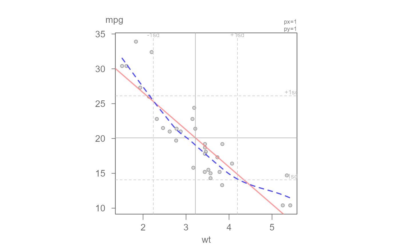 #> int wt^1
#> 37.285126 -5.344472
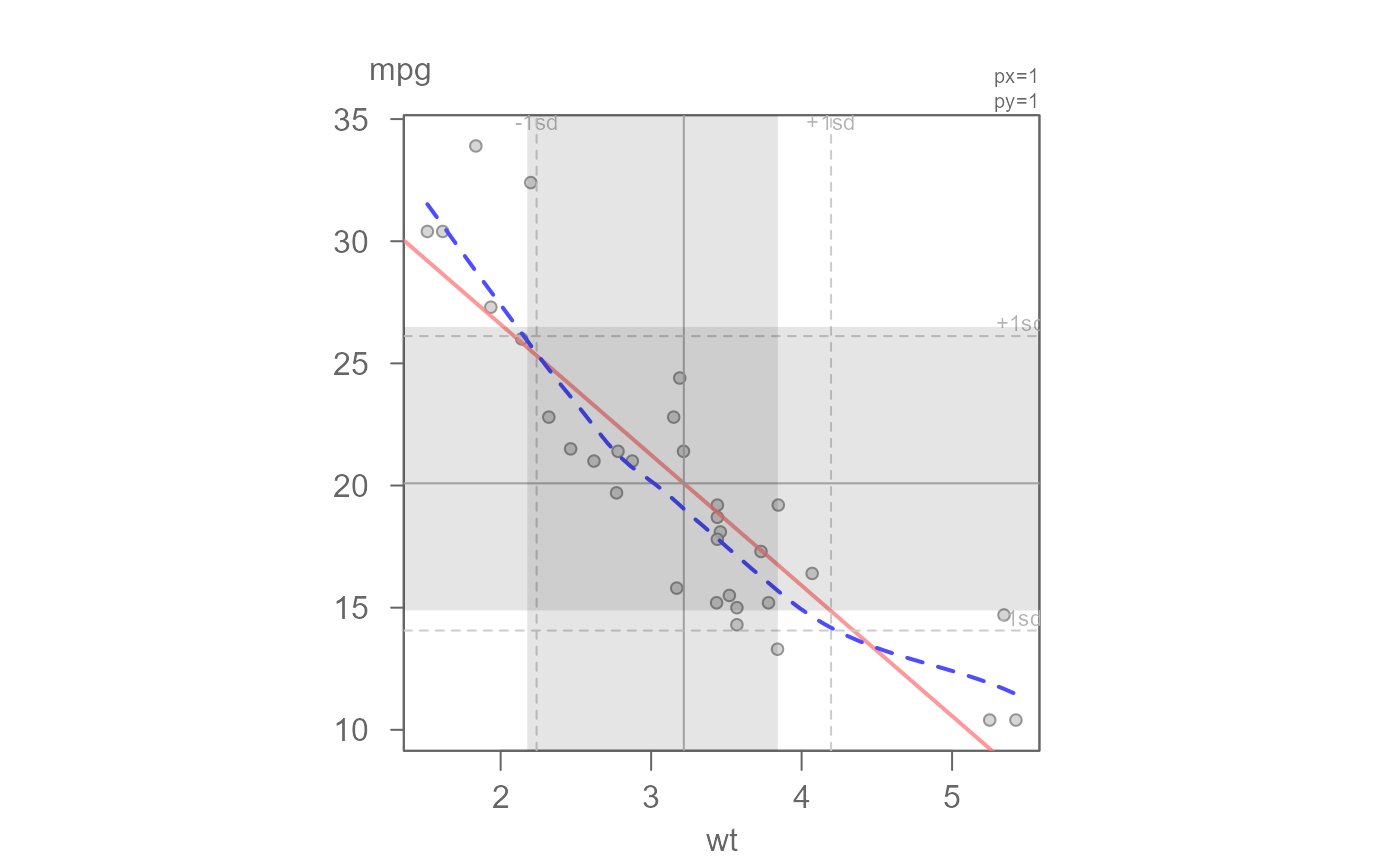
# Add the inner 68% quantile to compare the true 68% of data to the SD
eda_lm(mtcars, wt, mpg, loe = TRUE, q = TRUE)
#> int wt^1
#> 37.285126 -5.344472
# Add the inner 68% quantile to compare the true 68% of data to the SD
eda_lm(mtcars, wt, mpg, loe = TRUE, q = TRUE)
 #> int wt^1
#> 37.285126 -5.344472
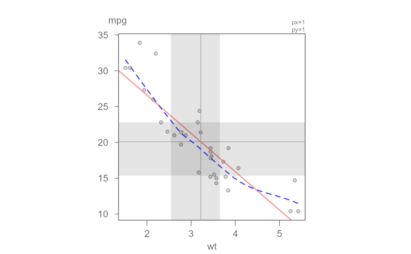
# Show the IQR box
eda_lm(mtcars, wt, mpg, loe = TRUE, q = TRUE, sd = FALSE, inner = 0.5)
#> int wt^1
#> 37.285126 -5.344472
# Show the IQR box
eda_lm(mtcars, wt, mpg, loe = TRUE, q = TRUE, sd = FALSE, inner = 0.5)
 #> int wt^1
#> 37.285126 -5.344472
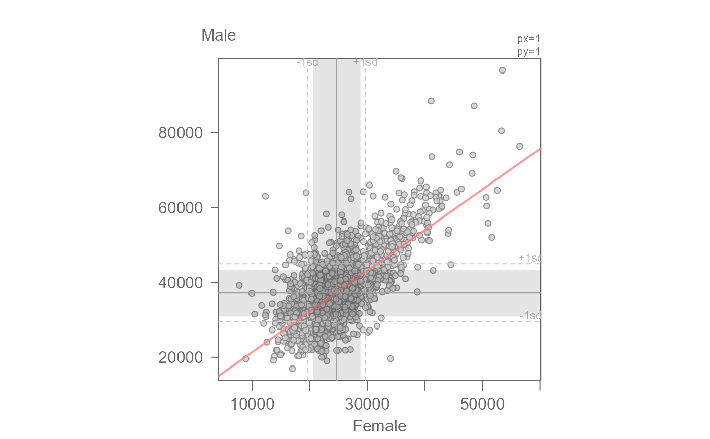
# Fit an OLS to income for Female vs Male
inc <- read.csv("https://mgimond.github.io/ES218/Data/Income_education.csv")
eda_lm(inc, x=B20004013, y = B20004007, xlab = "Female", ylab = "Male",
loe = TRUE)
#> int wt^1
#> 37.285126 -5.344472
# Fit an OLS to income for Female vs Male
inc <- read.csv("https://mgimond.github.io/ES218/Data/Income_education.csv")
eda_lm(inc, x=B20004013, y = B20004007, xlab = "Female", ylab = "Male",
loe = TRUE)
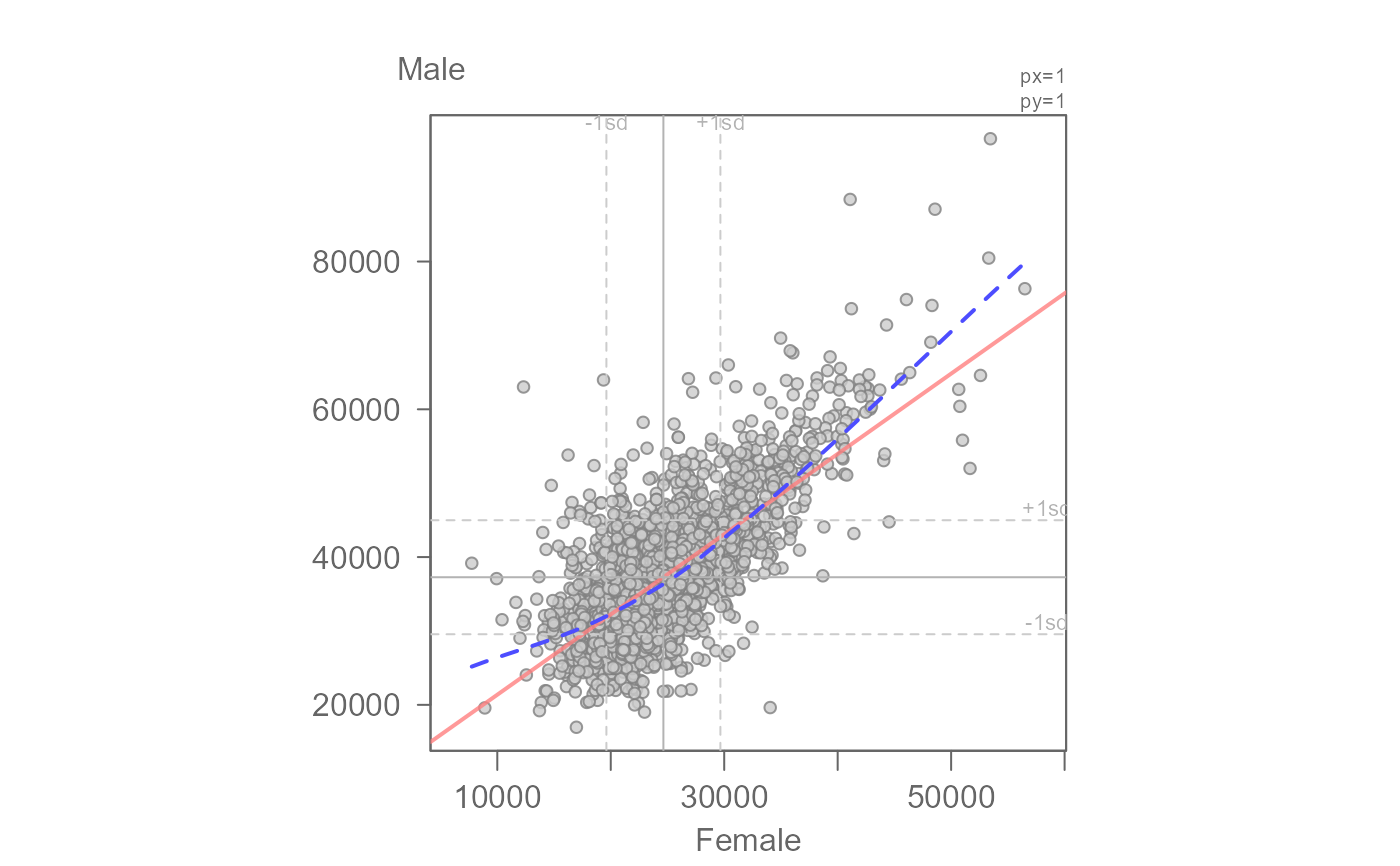 #> int Female^1
#> 10503.090485 1.086416
# Add the inner 68% quantile to compare the true 68% of data to the SD
eda_lm(inc, x = B20004013, y = B20004007, xlab = "Female", ylab = "Male",
q = TRUE)
#> int Female^1
#> 10503.090485 1.086416
# Add the inner 68% quantile to compare the true 68% of data to the SD
eda_lm(inc, x = B20004013, y = B20004007, xlab = "Female", ylab = "Male",
q = TRUE)
 #> int Female^1
#> 10503.090485 1.086416
# Apply a transformation to x and y axes: x -> 1/3 and y -> log
eda_lm(inc, x = B20004013, y = B20004007, px = 1/3, py = 0, loe = TRUE,
xlab = expression(("Female income") ^ frac(1,3)),
ylab = "log(Male income)")
#> int Female^1
#> 10503.090485 1.086416
# Apply a transformation to x and y axes: x -> 1/3 and y -> log
eda_lm(inc, x = B20004013, y = B20004007, px = 1/3, py = 0, loe = TRUE,
xlab = expression(("Female income") ^ frac(1,3)),
ylab = "log(Male income)")
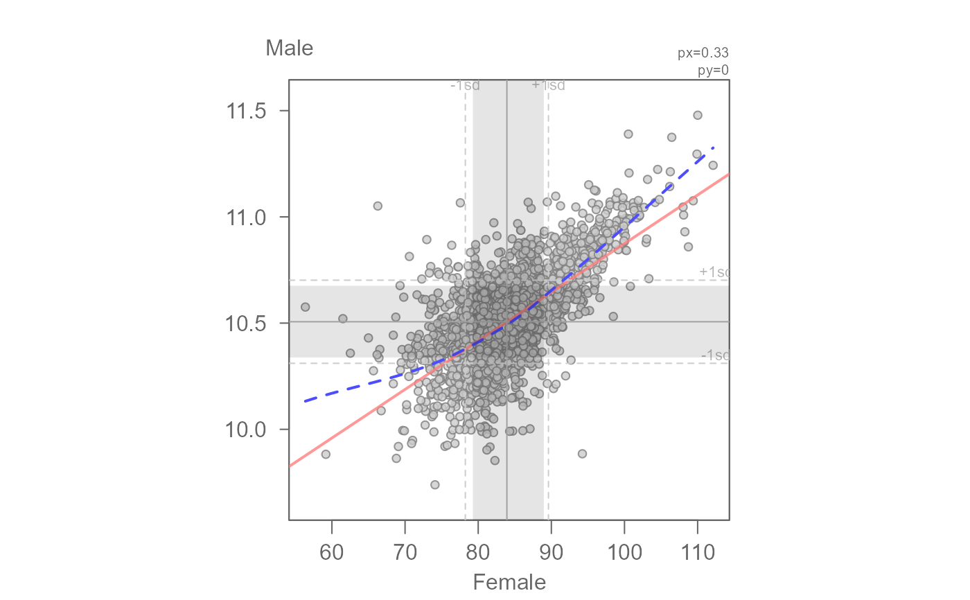 #> int ("Female income")^frac(1, 3)^1
#> 8.58646713 0.02287702
# You can opt to show the original values on scaled axes
eda_lm(inc, x = B20004013, y = B20004007, px = 1/3, py = 0, loe = TRUE,
xlab = "Female", ylab = "Male", raw_tick = TRUE)
#> Note: Scaled x-axis displays the untransformed values.
#> Note: Scaled y-axis displays the untransformed values.
#> int ("Female income")^frac(1, 3)^1
#> 8.58646713 0.02287702
# You can opt to show the original values on scaled axes
eda_lm(inc, x = B20004013, y = B20004007, px = 1/3, py = 0, loe = TRUE,
xlab = "Female", ylab = "Male", raw_tick = TRUE)
#> Note: Scaled x-axis displays the untransformed values.
#> Note: Scaled y-axis displays the untransformed values.
 #> int Female^1
#> 8.58646713 0.02287702
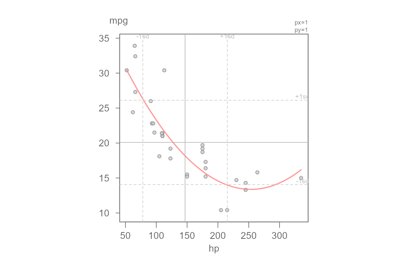
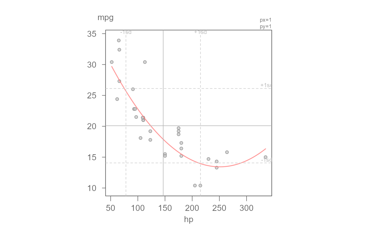
# Fit a second order polynomial
eda_lm(mtcars, hp, mpg, poly = 2)
#> int Female^1
#> 8.58646713 0.02287702
# Fit a second order polynomial
eda_lm(mtcars, hp, mpg, poly = 2)
 #> int hp^1 hp^2
#> 40.4091172029 -0.2133082599 0.0004208156
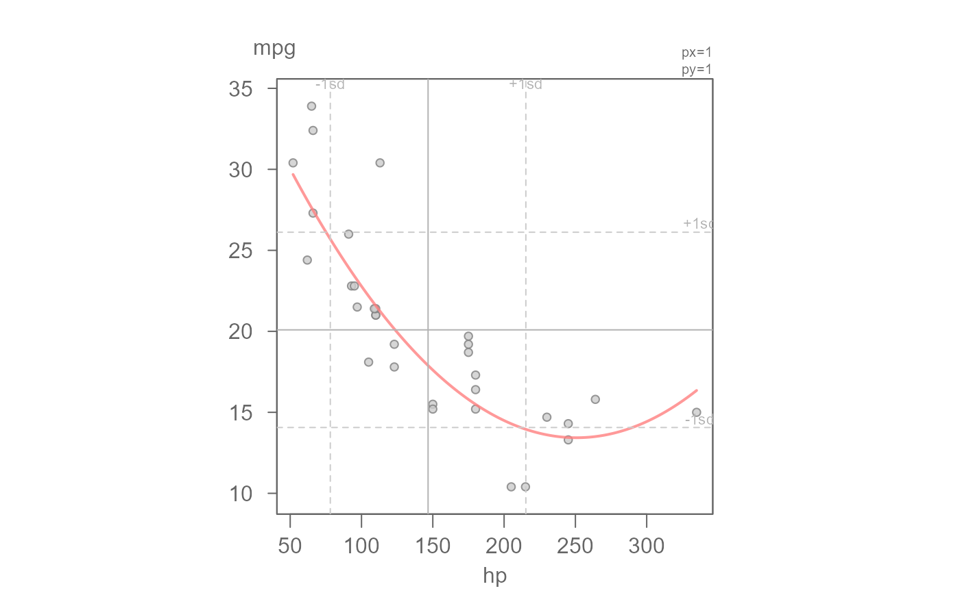
# Fit a robust regression model
eda_lm(mtcars, hp, mpg, robust = TRUE, poly = 2)
#> int hp^1 hp^2
#> 40.4091172029 -0.2133082599 0.0004208156
# Fit a robust regression model
eda_lm(mtcars, hp, mpg, robust = TRUE, poly = 2)
 #> int hp^1 hp^2
#> 39.3003734539 -0.2062942523 0.0004113048
#> int hp^1 hp^2
#> 39.3003734539 -0.2062942523 0.0004113048