eda_qqmat Generates a matrix of empirical QQ plots
Usage
eda_qqmat(
  dat,
  x,
  fac,
  p = 1L,
  tukey = FALSE,
  base = exp(1),
  q.type = 5,
  upper = FALSE,
  xylim = NULL,
  resid = FALSE,
  stat = mean,
  plot = TRUE,
  grey = 0.6,
  pch = 21,
  p.col = "grey40",
  p.fill = "grey60",
  size = 1,
  text.size = 1,
  tail.pch = 21,
  tail.p.col = "grey70",
  tail.p.fill = NULL,
  tic.size = 0.7,
  alpha = 0.8,
  q = FALSE,
  tails = FALSE,
  med = FALSE,
  inner = 0.75,
  ...
)
Arguments
- dat
Data frame.
- x
Continuous variable.
- fac
Categorical variable.
- p
Power transformation to apply to the continuous variable.
- tukey
Boolean determining if a Tukey transformation should be adopted (FALSE adopts a Box-Cox transformation).
- base
Base used with the log() function if
p = 0.- q.type
An integer between 1 and 9 selecting one of the nine quantile algorithms. (See
quantiletile function).- upper
Boolean determining if both upper and lower triangular matrix should be plotted. If set to
FALSE, only the lower triangular matrix is plotted.- xylim
X and Y axes limits.
- resid
Boolean determining if residuals should be plotted. Residuals are computed using the
statparameter.- stat
Statistic to use if residuals are to be computed. Currently
mean(default) ormedian.- plot
Boolean determining if plot should be generated.
- grey
Grey level to apply to plot elements (0 to 1 with 1 = black).
- pch
Point symbol type.
- p.col
Color for point symbol.
- p.fill
Point fill color passed to
bg(Only used forpchranging from 21-25).- size
Point symbol size (0-1).
- text.size
Size for category text in diagonal box.
- tail.pch
Tail-end point symbol type (See
tails).- tail.p.col
Tail-end color for point symbol (See
tails).- tail.p.fill
Tail-end point fill color passed to
bg(Only used fortail.pchranging from 21-25).- tic.size
Size of tic labels (defaults to 0.8).
- alpha
Point transparency (0 = transparent, 1 = opaque). Only applicable if
rgb()is not used to define point colors.- q
Boolean determining if grey box highlighting the
innerregion should be displayed.- tails
Boolean determining if points outside of the
innerregion should be symbolized differently. Tail-end points are symbolized via thetail.pch,tail.p.colandtail.p.fillarguments.- med
Boolean determining if median lines should be drawn.
- inner
Fraction of mid-values to highlight in
qortails. Defaults to the inner 75 percent of values.- ...
Not used
Value
Returns a list with the following components:
data: List with inputxandyvalues for each group. May be interpolated to smallest quantile batch if batch sizes don't match. Values will reflect power transformation defined inp.p: Transformation applied to original values.
Details
The function will generate an empirical QQ plot matrix. Most of the
arguments available in eda_qq are echoed in this function. The one
notable difference is the default settings. By default, eda_qqmat will
generate a plain vanilla set of plots.
The QQ plot matrix is most effective in comparing residuals after the data
are fitted by the mean or median. To plot the residuals, set
resid=TRUE. By default, the mean is used. You can change the
statistic to the median by setting stat=median.
The function also allows for batch transformation of values via the
p argument. The transformation is applied to the data prior to
computing the residuals.
References
John M. Chambers, William S. Cleveland, Beat Kleiner, Paul A. Tukey. Graphical Methods for Data Analysis (1983)
Examples
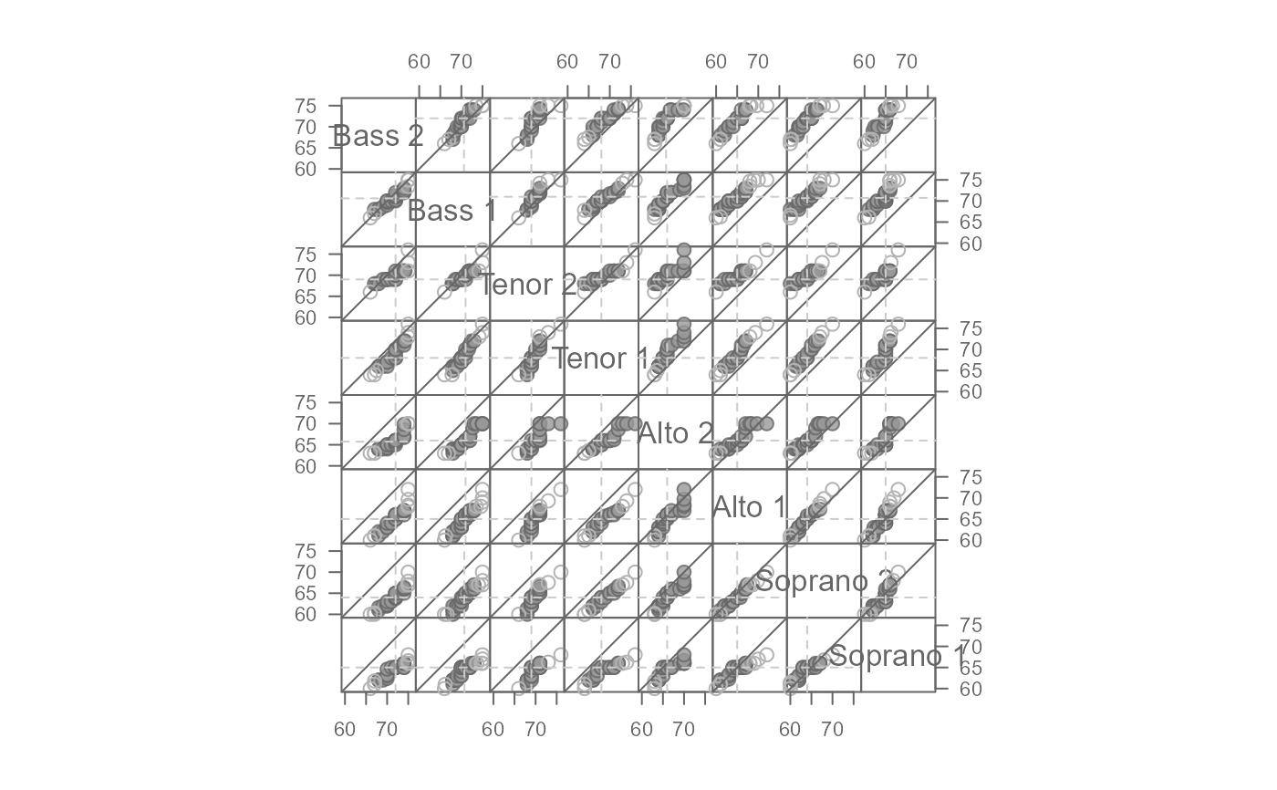
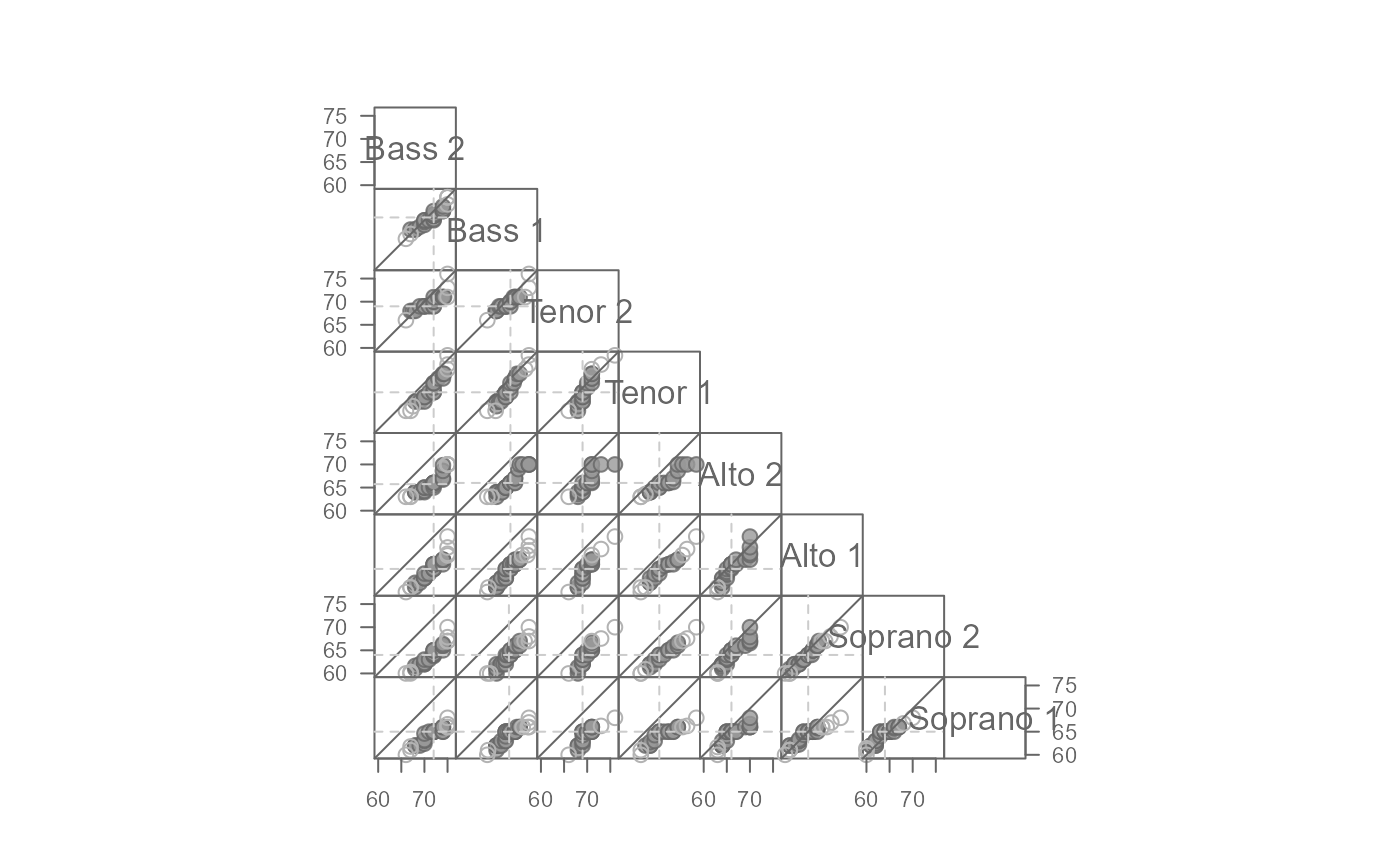
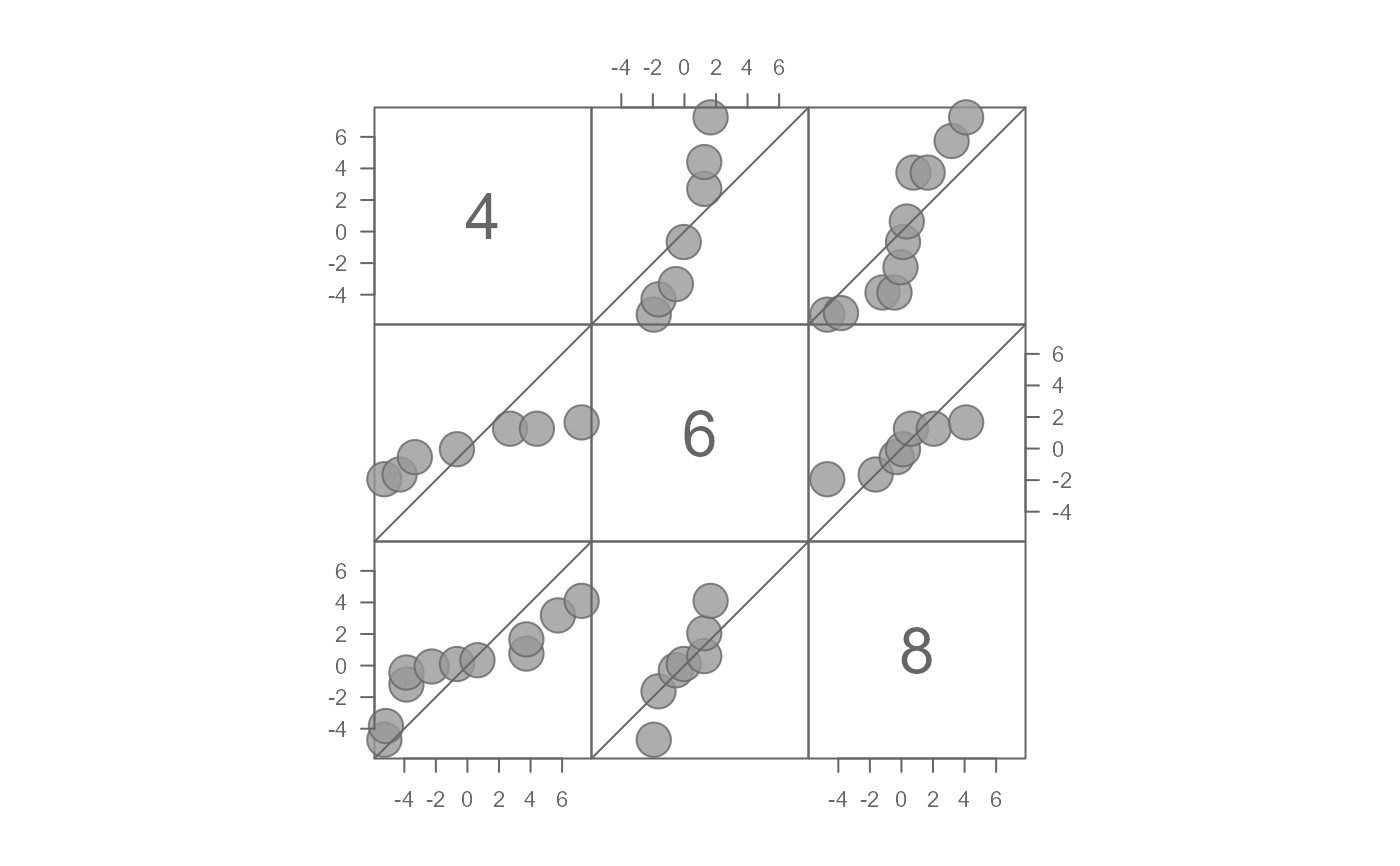
# Default output
singer <- lattice::singer
eda_qqmat(singer, height, voice.part)
 # Symbolize points outside of the "inner" region using an open point symbol
eda_qqmat(singer, height, voice.part, tails = TRUE)
# Symbolize points outside of the "inner" region using an open point symbol
eda_qqmat(singer, height, voice.part, tails = TRUE)
 # Set the inner region to cover 80% and change the outer point symbol to "+"
eda_qqmat(singer, height, voice.part, inner = 0.8, tails = TRUE, tail.pch = 3)
# Set the inner region to cover 80% and change the outer point symbol to "+"
eda_qqmat(singer, height, voice.part, inner = 0.8, tails = TRUE, tail.pch = 3)
 # Add the upper triangle to the matrix
eda_qqmat(singer, height, voice.part, upper = TRUE)
# Add the upper triangle to the matrix
eda_qqmat(singer, height, voice.part, upper = TRUE)
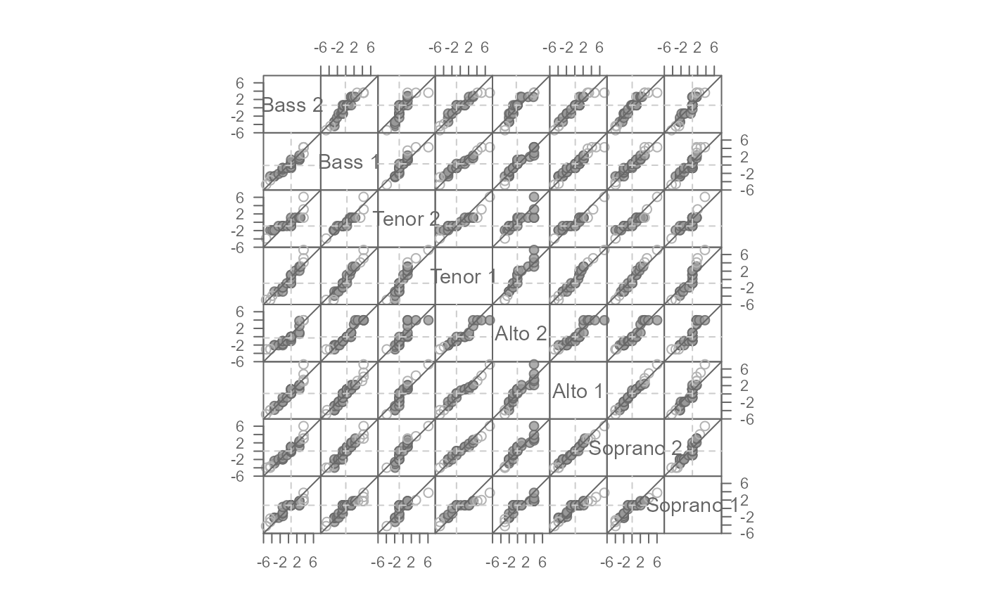
 # Plot residuals after fitting mean to each batch
eda_qqmat(singer, height, voice.part, resid = TRUE)
# Plot residuals after fitting mean to each batch
eda_qqmat(singer, height, voice.part, resid = TRUE)
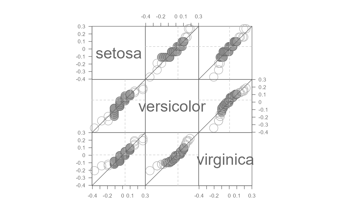 # Log transform the data, then plot the residuals after fitting the mean model
eda_qqmat(iris, Petal.Length, Species, resid = TRUE, p = 0)
#> Note that a power transformation of 0 was applied to the data before they were processed for the plot.
# Log transform the data, then plot the residuals after fitting the mean model
eda_qqmat(iris, Petal.Length, Species, resid = TRUE, p = 0)
#> Note that a power transformation of 0 was applied to the data before they were processed for the plot.
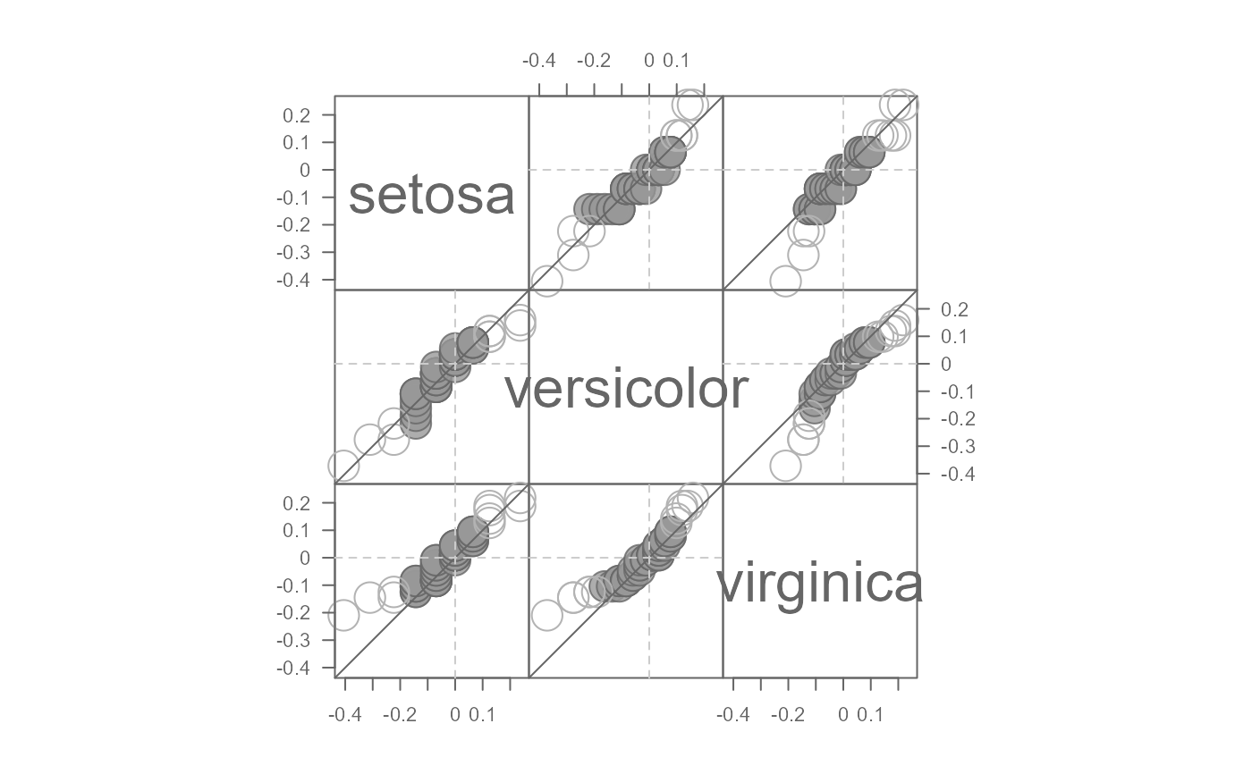 # Fit the median model instead of the mean
eda_qqmat(iris, Petal.Length, Species, resid = TRUE, p = 0, stat = median)
#> Note that a power transformation of 0 was applied to the data before they were processed for the plot.
# Fit the median model instead of the mean
eda_qqmat(iris, Petal.Length, Species, resid = TRUE, p = 0, stat = median)
#> Note that a power transformation of 0 was applied to the data before they were processed for the plot.
 # Shade the "inner" regions (defaults to the mid 70% of values)
eda_qqmat(iris, Petal.Length, Species, resid = TRUE, q = TRUE, p = 0)
#> Note that a power transformation of 0 was applied to the data before they were processed for the plot.
# Shade the "inner" regions (defaults to the mid 70% of values)
eda_qqmat(iris, Petal.Length, Species, resid = TRUE, q = TRUE, p = 0)
#> Note that a power transformation of 0 was applied to the data before they were processed for the plot.
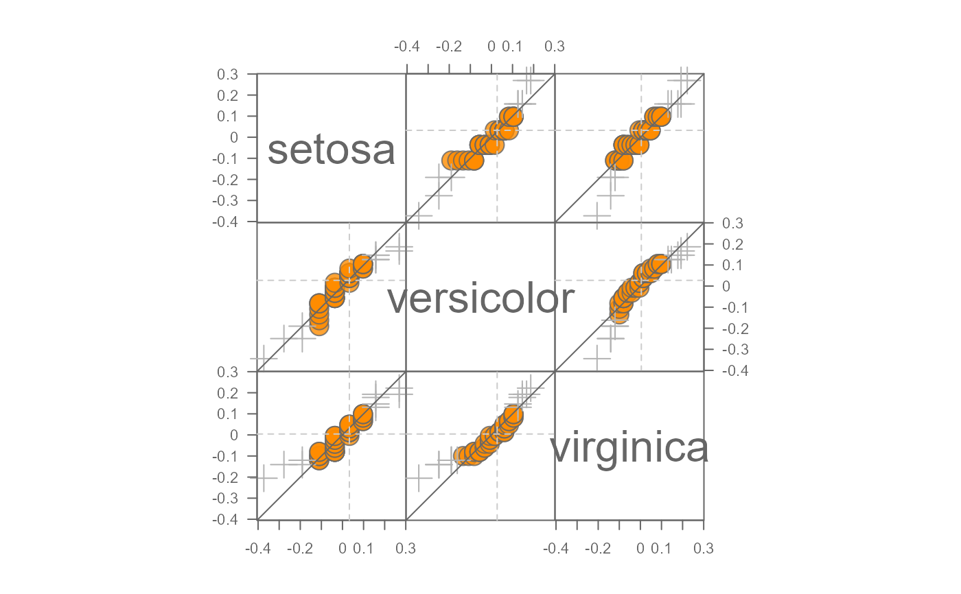
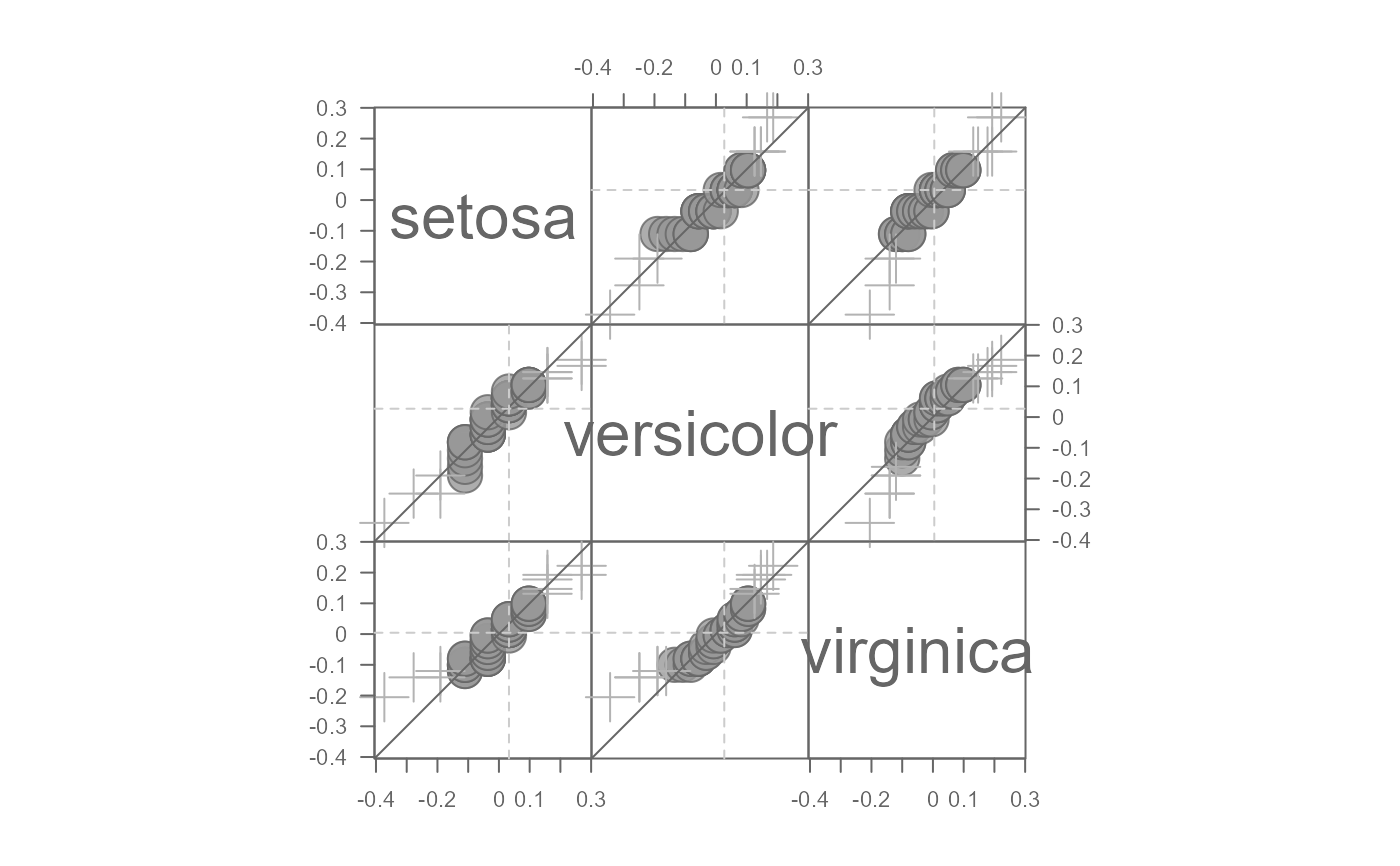 # Change inner region point symbols to dark orange and change inner region
# range to cover 90% of mid values
eda_qqmat(iris, Petal.Length, Species, resid = TRUE, p = 0, inner = 0.9,
tail.pch = 3, p.fill = "orange2")
#> Note that a power transformation of 0 was applied to the data before they were processed for the plot.
# Change inner region point symbols to dark orange and change inner region
# range to cover 90% of mid values
eda_qqmat(iris, Petal.Length, Species, resid = TRUE, p = 0, inner = 0.9,
tail.pch = 3, p.fill = "orange2")
#> Note that a power transformation of 0 was applied to the data before they were processed for the plot.