The eda_sl function generates William Cleveland's
spread-location plot for univariate and bivariate data. The function will also
generate Tukeys' spread-level plot.
Usage
eda_sl(
  dat,
  x = NULL,
  fac = NULL,
  type = "location",
  p = 1,
  tukey = FALSE,
  base = exp(1),
  sprd = "frth",
  jitter = 0.01,
  robust = TRUE,
  loess.d = list(family = "symmetric", degree = 1, span = 1),
  label = TRUE,
  label.col = "lightsalmon",
  xlab = NULL,
  ylab = NULL,
  labelxbuff = 0.05,
  labelybuff = 0.05,
  show.par = FALSE,
  plot = TRUE,
  ...
)
Arguments
- dat
Dataframe of univariate data or a linear model.
- x
Continuous variable column (ignored if
datis a linear model).- fac
Categorical variable column (ignored if
datis a linear model).- type
s-l plot type.
"location"= spread-location,"level"= spread-level (only for univariate data)."dependence"= spread-dependence (only for bivariate model input).- p
Power transformation to apply to variable. Ignored if input is a linear model.
- tukey
Logical; Determines if a Tukey transformation should be adopted (FALSE adopts a Box-Cox transformation).
- base
Base used with the
log()function ifpxorpyis0.- sprd
Choice of spreads used in the spread-versus-level plot (i.e. when
type = "level"). Either interquartile,sprd = "IQR"or fourth-spread,sprd = "frth"(default).- jitter
Jittering parameter for the spread-location plot. A fraction of the range of location values.
- robust
Logical; Indicates if robust regression should be used on the spread-level plot.
- loess.d
Arguments passed to the internal loess function. Applies only to the bivariate model s-l plots and the spread-level plot.
- label
Logical; Determines if group labels are to be added to the spread-location plot.
- label.col
Color assigned to group labels (only applicable if
type = location).- xlab
X label for output plot.
- ylab
Y label for output plot.
- labelxbuff
Buffer to add to the edges of the plot to make room for the labels in a spread-location plot. Value is a fraction of the plot width.
- labelybuff
Buffer to add to the top of the plot to make room for the labels in a spread-location plot. Value is a fraction of the plot width.
- show.par
Boolean determining if the power transformation applied to the data should be displayed.
- plot
Logical; Determines if plot should be generated.
- ...
Arguments passed on to
.eda_plot_xyyA numeric vector or column name in
datfor the y-axis.pxPower transformation used in the input data to display if
show.par = TRUE.pyPower transformation used in the input data to display if
show.par = TRUE.raw_tickLogical. If
TRUE, original (untransformed) equally spaced tick values are displayed on the re-expressed axes.xlimX-axis range.
ylimY-axis range.
regLogical; whether to fit and display a regression line.
polyInteger; regression model polynomial degree (defaults to 1 for linear model).
rlm.dList; parameters for
MASS::rlm, (e.g.,list(psi = "psi.bisquare")).wOptional numeric vector of weights for regression.
lm.colRegression line color.
lm.lwNumeric; Regression line width.
lm.ltyNumeric; Regression line type.
sdLogical; whether to show ±1 SD lines.
mean.lLogical; whether to show x and y mean reference lines.
aspLogical; whether to preserve the aspect ratio (ignored if
square = FALSE).squareLogical; whether to create a square plotting window.
greyNumeric between
0-1; controls grayscale background elements (0 = black,1 = white).pchInteger; point symbol.
p.colPoint border color.
p.fillPoint fill color.
sizePoint size.
alphaPoint transparency level (0 = 100\% transparent, 1 = 100\% opaque).
qLogical; whether to draw inner quantile boxes (quantile shading).
q.typeInteger; type of quantile calculation (see
quantile).innerNumeric; defines the inner fraction of values to highlight with quantile shading.
qcolFill color of quantile shading.
loeLogical; whether to plot loess smooth line.
loe.lwNumeric; Loess smooth line width.
loe.colLoess smooth color.
loe.ltyNumeric; Loess smooth line type.
statsLogical; if
TRUE, displays model statistics (R², β, p-value).stat.sizeText size for
statsplot display.hlineNumeric; location(s) of additional horizontal reference lines. Can be passed via the
c()function.vlineNumeric; location(s) of additional vertical reference lines. Can be passed via the
c()function.
Details
The function generates a few variations of the spread-location/spread-level
plots depending on the data input type and parameter passed to the
type argument. The residual spreads are mapped to the y-axis and the
levels are mapped to the x-axis. Their values are computed as follows:
type = "location"(univariate data):
William Cleveland's spread-location plot applied to univariate data.
\(\ spread = \sqrt{|residuals|}\)
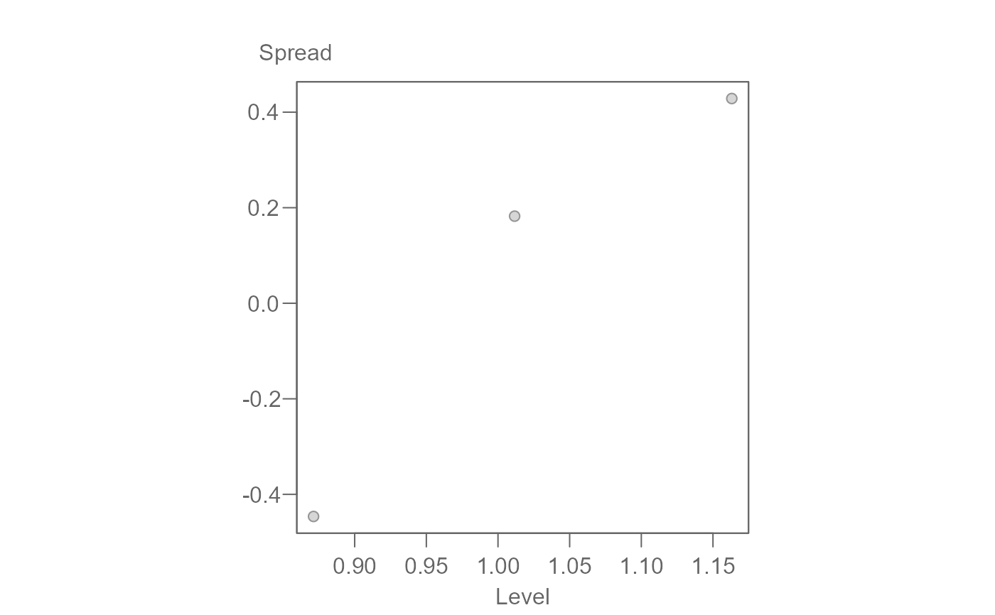
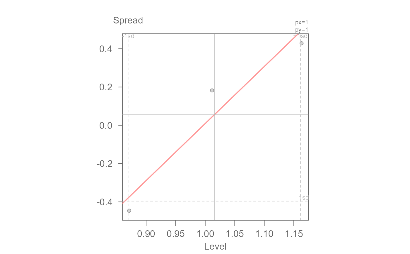
\(\ location = medians\)type = "level"(univariate data):
Tukey's spread-level plot (aka spread-versus-level plot, Hoaglin et al., p 260). If the pattern is close to linear, the plot can help find a power transformation that will help stabilize the spread in the data by subtracting one from the fitted slope. This option outputs the slope of the fitted line in the console. A loess is added to assess linearity. By default, the fourth spread is used to define the spread. Alternatively, the IQR can be used by settingspread = "IQR". The output will be nearly identical except for small datasets where the two methods may diverge slightly in output.
\(\ spread = log(fourth\ spread(residuals))\)
\(\ location = log(medians)\)type = "location"if input is a model of classlm,eda_lmoreda_rline:
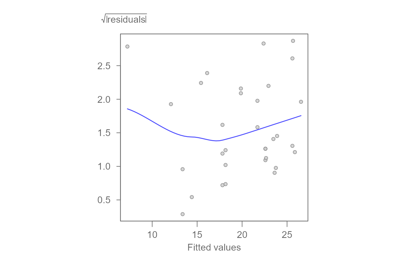
William Cleveland's spread-location plot (aka scale-location plot) applied to residuals of a linear model.
\(\ spread = \sqrt{|residuals|}\)
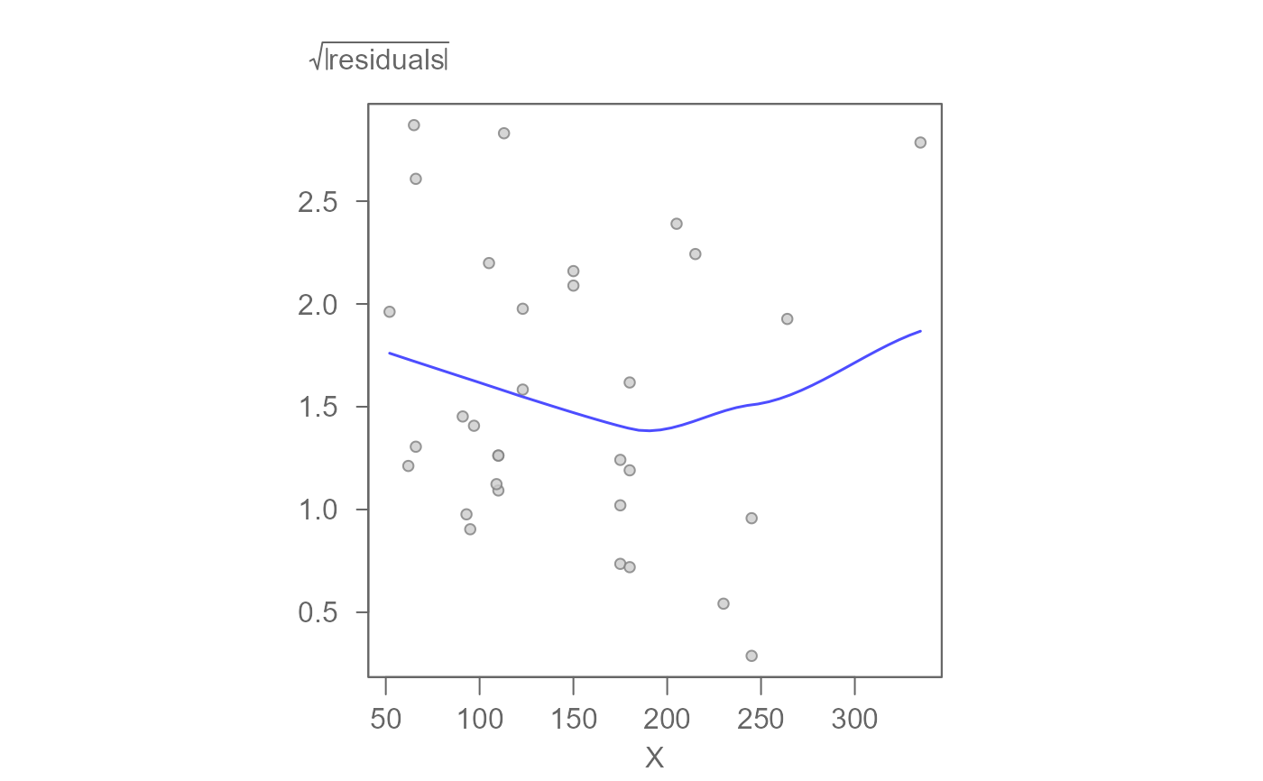
\(\ location = fitted\ values\)type = "dependence"if input is a model of classlm,eda_lmoreda_rline:
William Cleveland's spread-location plot applied to residuals of a linear model.
\(\ spread = \sqrt{|residuals|}\)
\(\ dependence = x\ variable\)
References
Understanding Robust and Exploratory Data Analysis, Hoaglin, David C., Frederick Mosteller, and John W. Tukey, 1983.
William S. Cleveland. Visualizing Data. Hobart Press (1993)
Examples
cars <- MASS::Cars93
# Cleveland's spread-location plot applied to univariate data
eda_sl(cars, MPG.city, Type)
 # You can specify the exact form of the spread on the y-axis
# via the ylab argument
eda_sl(cars, MPG.city, Type, ylab = expression(sqrt(abs(residuals))) )
# You can specify the exact form of the spread on the y-axis
# via the ylab argument
eda_sl(cars, MPG.city, Type, ylab = expression(sqrt(abs(residuals))) )
 # The function can also generate Tukey's spread-level plot to identify a
# power transformation that can stabilize spread across fitted values
# following power = 1 - slope
eda_sl(cars, MPG.city, Type, type = "level")
# The function can also generate Tukey's spread-level plot to identify a
# power transformation that can stabilize spread across fitted values
# following power = 1 - slope
eda_sl(cars, MPG.city, Type, type = "level")
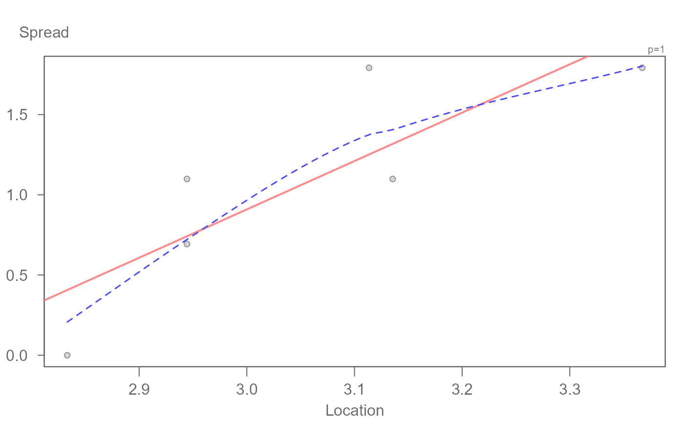 #> int Location^1
#> -8.009091 2.969832
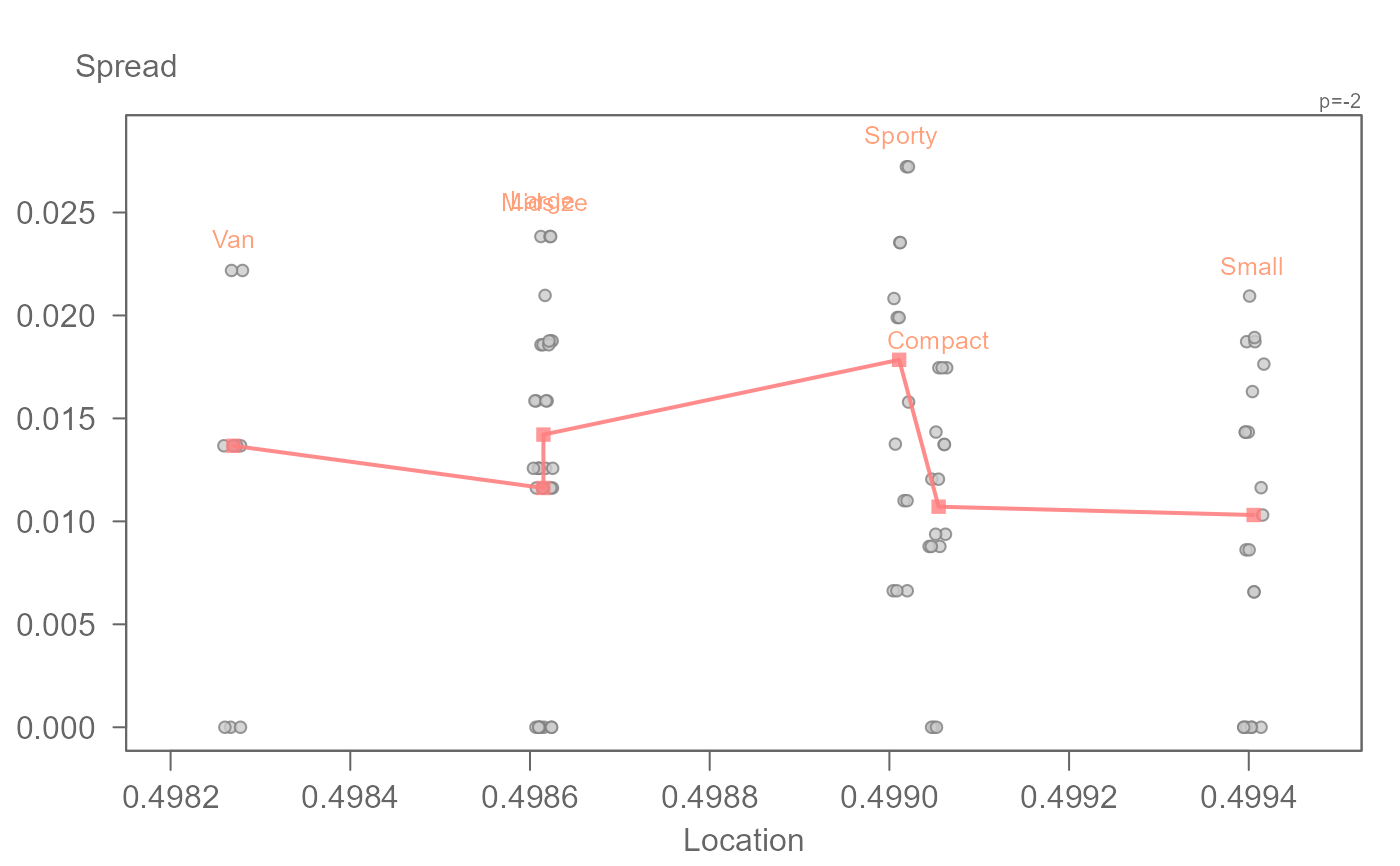
# A slope of around 3 is computed from the s-l plot, therefore, a suggested
# power is 1 - 3 = -2. We can apply a power transformation within the
# function via the p argument. By default, a Box-Cox transformation method
# is adopted.
eda_sl(cars, MPG.city, Type, p = -2)
#> int Location^1
#> -8.009091 2.969832
# A slope of around 3 is computed from the s-l plot, therefore, a suggested
# power is 1 - 3 = -2. We can apply a power transformation within the
# function via the p argument. By default, a Box-Cox transformation method
# is adopted.
eda_sl(cars, MPG.city, Type, p = -2)
 # Spread-location plot can also be generated from residuals of a linear model
M1 <- lm(mpg ~ hp, mtcars)
eda_sl(M1)
# Spread-location plot can also be generated from residuals of a linear model
M1 <- lm(mpg ~ hp, mtcars)
eda_sl(M1)
 # Spread can be compared to X instead of fitted value
eda_sl(M1, type = "dependence")
# Spread can be compared to X instead of fitted value
eda_sl(M1, type = "dependence")