eda_theo generates a theoretical QQ plot for many common
distributions including the Normal, uniform and gamma distributions.
Usage
eda_theo(
  x,
  p = 1L,
  tukey = FALSE,
  base = exp(1),
  q.type = 5,
  dist = "norm",
  dist.l = list(),
  resid = FALSE,
  stat = mean,
  plot = TRUE,
  show.par = TRUE,
  grey = 0.6,
  pch = 21,
  p.col = "grey50",
  p.fill = "grey80",
  size = 1,
  alpha = 0.8,
  med = TRUE,
  q = FALSE,
  iqr = TRUE,
  grid = FALSE,
  tails = FALSE,
  inner = 0.75,
  tail.pch = 21,
  tail.p.col = "grey70",
  tail.p.fill = NULL,
  xlab = NULL,
  ylab = NULL,
  title = NULL,
  t.size = 1.2,
  ...
)
Arguments
- x
Vector of continuous values.
- p
Power transformation to apply to
x.- tukey
Boolean determining if a Tukey transformation should be adopted (FALSE adopts a Box-Cox transformation).
- base
Base used with the log() function if
p = 0.- q.type
An integer between 4 and 9 selecting one of the nine quantile algorithms. (See the
eda_fvalfunction).- dist
Choice of theoretical distribution.
- dist.l
List of parameters passed to the distribution quantile function.
- resid
Boolean determining if residuals should be plotted. Residuals are computed using the
statparameter.- stat
Statistic to use if residuals are to be computed. Currently
mean(default) ormedian.- plot
Boolean determining if plot should be generated.
- show.par
Boolean determining if parameters such as power transformation or formula should be displayed.
- grey
Grey level to apply to plot elements (0 to 1 with 1 = black).
- pch
Point symbol type.
- p.col
Color for point symbol.
- p.fill
Point fill color passed to
bg(Only used forpchranging from 21-25).- size
Point size (0-1)
- alpha
Point transparency (0 = transparent, 1 = opaque). Only applicable if
rgb()is not used to define point colors.- med
Boolean determining if median lines should be drawn.
- q
Boolean determining if
innerdata region should be shaded.- iqr
Boolean determining if an IQR line should be fitted to the points.
- grid
Boolean determining if a grid should be added.
- tails
Boolean determining if points outside of the
innerregion should be symbolized differently. Tail-end points are symbolized via thetail.pch,tail.p.colandtail.p.fillarguments.- inner
Fraction of the data considered as "mid values". Defaults to 75%. Used to define shaded region boundaries,
q, or to identify which of the tail-end points are to be symbolized differently,tails.- tail.pch
Tail-end point symbol type (See
tails).- tail.p.col
Tail-end color for point symbol (See
tails).- tail.p.fill
Tail-end point fill color passed to
bg(Only used fortail.pchranging from 21-25).- xlab
X label for output plot.
- ylab
Y label for output plot.
- title
Title to add to plot.
- t.size
Title size.
- ...
Not used
Value
A dataframe with the input vector elements and matching theoretical
quantiles. Any transformation applied to x is reflected in the
output.
Details
The function generates a theoretical QQ plot.
Currently, only the Normal QQ plot (dist="norm"), exponential
QQ plot (dist="exp"), uniform QQ plot (dist="unif"),
gamma QQ plot (dist="gamma"), chi-squared QQ plot
(dist="chisq"), and the Weibull QQ plot (dist="weibull") are
supported. By default, the Normal QQ plot maps the unit Normal
quantiles to the x-axis (i.e. centered on a mean of 0 and standard deviation
of 1 unit).
Note that arguments can be passed to the respective quantile functions via
the d.list argument. Some quantile functions require at least one
argument. For example, the qgamma function requires that the shape
parameter be specified and the qchisq function requires that the
degrees of freedom, df, be specified. See examples.
References
John M. Chambers, William S. Cleveland, Beat Kleiner, Paul A. Tukey. Graphical Methods for Data Analysis (1983)
Examples
singer <- lattice::singer
bass2 <- subset(singer, voice.part == "Bass 2", select = height, drop = TRUE )
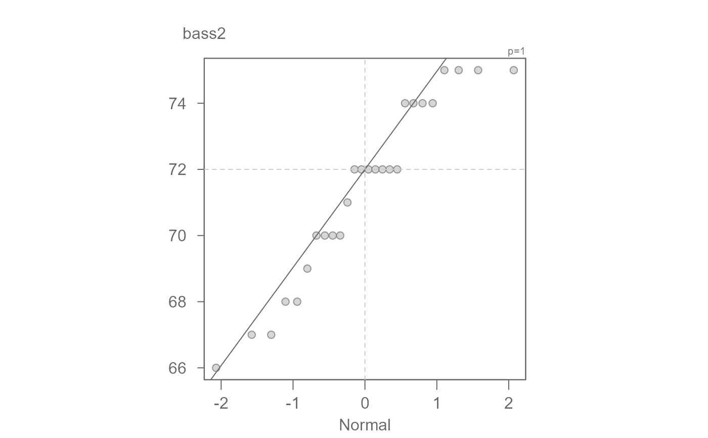
# Generate a normal QQ plot
eda_theo(bass2)
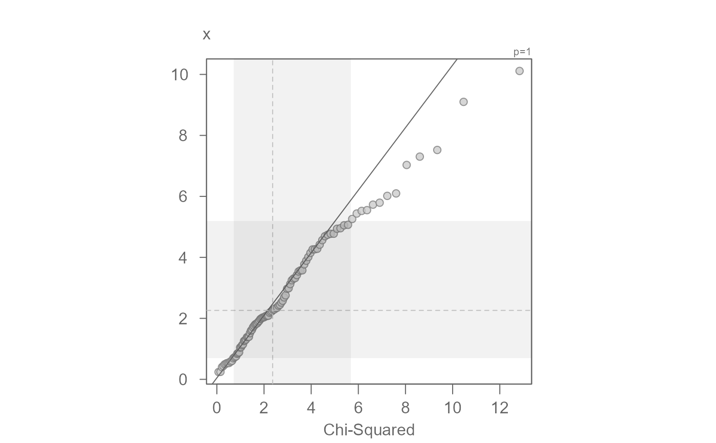
 # Generate a chi-squared QQ plot. The distribution requires that the degrees
# of freedom be specified. The inner 70% shaded region is added.
set.seed(270); x <- rchisq(100, df =3)
eda_theo(x, dist = "chisq", dist.l = list(df = 3), q = TRUE)
# Generate a chi-squared QQ plot. The distribution requires that the degrees
# of freedom be specified. The inner 70% shaded region is added.
set.seed(270); x <- rchisq(100, df =3)
eda_theo(x, dist = "chisq", dist.l = list(df = 3), q = TRUE)
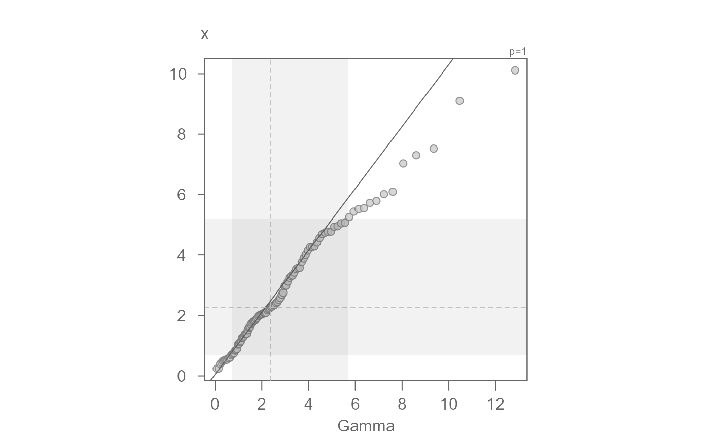
 # Generate a gamma QQ plot. Note that gamma requires at the very least the
# shape parameter. The chi-squared distribution is a special case of the
# gamma distribution where shape = df/2 and rate = 1/2.
eda_theo(x, dist = "gamma", dist.l = list(shape = 3/2, rate = 1/2), q = TRUE)
# Generate a gamma QQ plot. Note that gamma requires at the very least the
# shape parameter. The chi-squared distribution is a special case of the
# gamma distribution where shape = df/2 and rate = 1/2.
eda_theo(x, dist = "gamma", dist.l = list(shape = 3/2, rate = 1/2), q = TRUE)
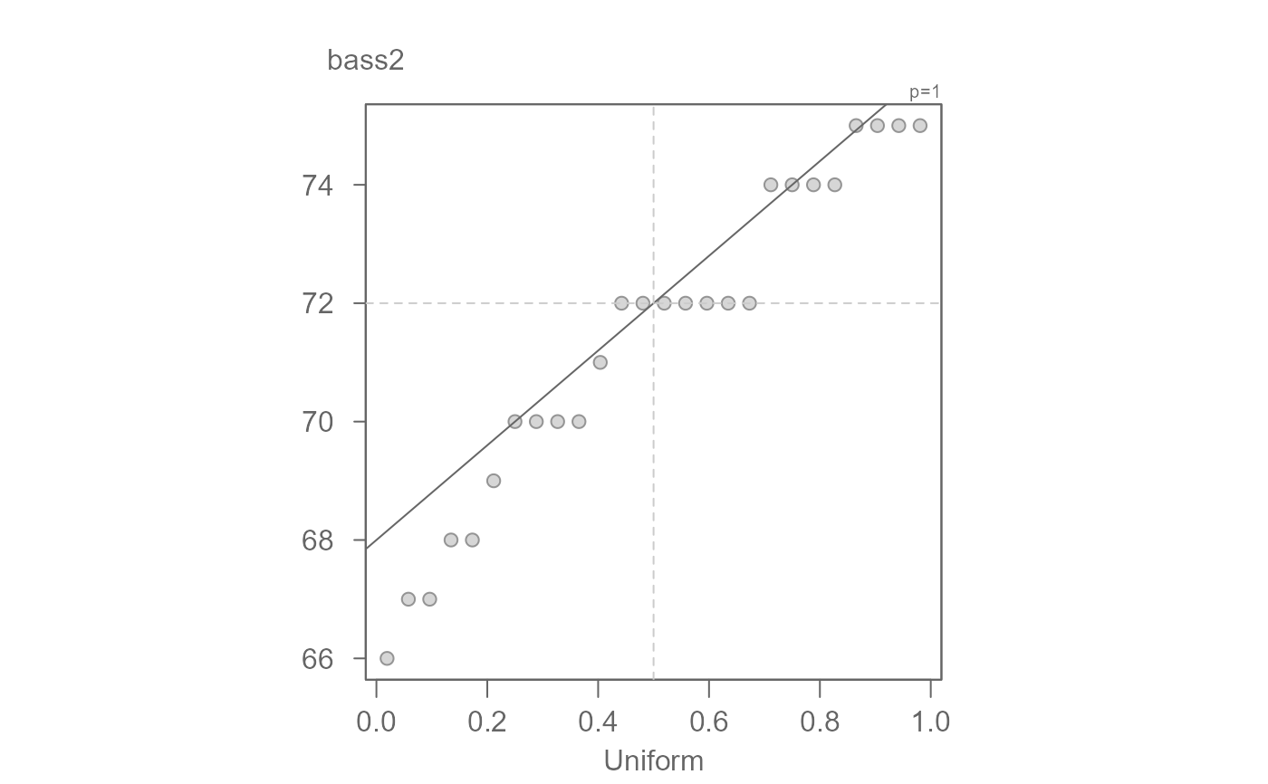
 # Generate a uniform QQ plot
eda_theo(bass2, dist = "unif")
# Generate a uniform QQ plot
eda_theo(bass2, dist = "unif")
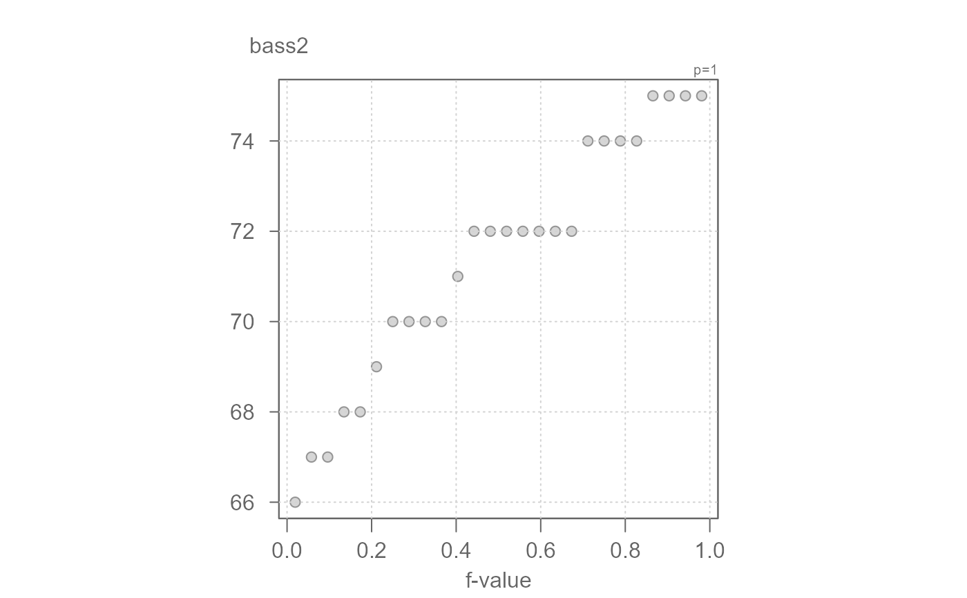
 # The uniform QQ plot can double as a quantile plot
eda_theo(bass2, dist = "unif", q = FALSE, med = FALSE,
iqr = FALSE, grid = TRUE, xlab = "f-value")
# The uniform QQ plot can double as a quantile plot
eda_theo(bass2, dist = "unif", q = FALSE, med = FALSE,
iqr = FALSE, grid = TRUE, xlab = "f-value")