eda_rline is an R implementation of Hoaglin, Mosteller
and Tukey's resistant line technique outlined in chapter 5 of
"Understanding Robust and Exploratory Data Analysis" (Wiley, 1983).
Usage
eda_rline(
  dat,
  x,
  y,
  px = 1,
  py = 1,
  tukey = FALSE,
  maxiter = 20,
  base = exp(1)
)
Arguments
- dat
Data frame.
- x
Column assigned to the x axis.
- y
Column assigned to the y axis.
- px
Power transformation to apply to the x-variable.
- py
Power transformation to apply to the y-variable.
- tukey
Logical; determining if a Tukey transformation should be adopted. (FALSE adopts a Box-Cox transformation).
- maxiter
Maximum number of iterations to run.
- base
Base used with the log() function if
pxorpyis0.
Value
Returns a list of class eda_rline with the following named
components:
data: Input data table with residualsa: Interceptb: Sloperesiduals: Residuals sorted on x-valuesx: Sorted x valuesy: y values following sorted x-valuesxmed: Median x values for each thirdymed: Median y values for each thirdindex: Index of sorted x values defining upper boundaries of each thirdsxlab: X label nameylab: Y label nameiter: Number of iterationsfitted.values: Fitted values
Details
This is an R implementation of the RLIN.F FORTRAN code in
Velleman et. al's book. This function fits a robust line using a
three-point summary strategy whereby the data are split into three equal
length groups along the x-axis and a line is fitted to the medians defining
each group via an iterative process. This function should mirror the
built-in stat::line function in its fitting strategy but it outputs
additional parameters.
See the accompanying resistant line
article for a detailed breakdown of the resistant line technique.
References
Velleman, P. F., and D. C. Hoaglin. 1981. Applications, Basics and Computing of Exploratory Data Analysis. Boston: Duxbury Press.
D. C. Hoaglin, F. Mosteller, and J. W. Tukey. 1983. Understanding Robust and Exploratory Data Analysis. Wiley.
Examples
# This first example uses breast cancer data from "ABC's of EDA" page 127.
# The output model's parameters should closely match: Y = -46.19 + 2.89X
# The plots shows the original data with a fitted resistant line (red)
# and a regular lm fitted line (dashed line), and the modeled residuals.
# The 3-point summary dots are shown in red.
M <- eda_rline(neoplasms, Temp, Mortality)
M
#> $data
#> Temp Mortality residuals
#> 1 31.8 67.3 21.59489403
#> 2 34.0 52.5 0.43651252
#> 3 40.2 68.1 -1.88256262
#> 4 42.1 84.6 9.12610790
#> 5 42.3 65.1 -10.95192678
#> 6 43.5 72.2 -7.32013487
#> 7 44.2 81.7 0.15674374
#> 8 45.1 89.2 5.05558767
#> 9 46.3 78.9 -8.71262042
#> 10 47.3 88.6 -1.90279383
#> 11 47.8 95.0 3.05211946
#> 12 48.5 87.0 -6.97100193
#> 13 49.2 95.9 -0.09412331
#> 14 49.9 104.5 6.48275530
#> 15 50.0 100.4 2.09373796
#> 16 51.3 102.5 0.43651252
#>
#> $b
#> [1] 2.890173
#>
#> $a
#> [1] -46.20241
#>
#> $residuals
#> [1] 21.59489403 0.43651252 -1.88256262 9.12610790 -10.95192678
#> [6] -7.32013487 0.15674374 5.05558767 -8.71262042 -1.90279383
#> [11] 3.05211946 -6.97100193 -0.09412331 6.48275530 2.09373796
#> [16] 0.43651252
#>
#> $x
#> [1] 31.8 34.0 40.2 42.1 42.3 43.5 44.2 45.1 46.3 47.3 47.8 48.5 49.2 49.9 50.0
#> [16] 51.3
#>
#> $y
#> [1] 67.3 52.5 68.1 84.6 65.1 72.2 81.7 89.2 78.9 88.6 95.0 87.0
#> [13] 95.9 104.5 100.4 102.5
#>
#> $xmed
#> [1] 40.2 45.7 49.9
#>
#> $ymed
#> [1] 67.30 85.15 100.40
#>
#> $index
#> [1] 5 11 16
#>
#> $xlab
#> [1] "Temp"
#>
#> $ylab
#> [1] "Mortality"
#>
#> $px
#> [1] 1
#>
#> $py
#> [1] 1
#>
#> $tukey
#> [1] FALSE
#>
#> $base
#> [1] 2.718282
#>
#> $iter
#> [1] 4
#>
#> $fitted.values
#> [1] 45.70511 52.06349 69.98256 75.47389 76.05193 79.52013 81.54326
#> [8] 84.14441 87.61262 90.50279 91.94788 93.97100 95.99412 98.01724
#> [15] 98.30626 102.06349
#>
#> attr(,"class")
#> [1] "eda_rline"
# Plot the output (red line is the resistant line)
plot(M)
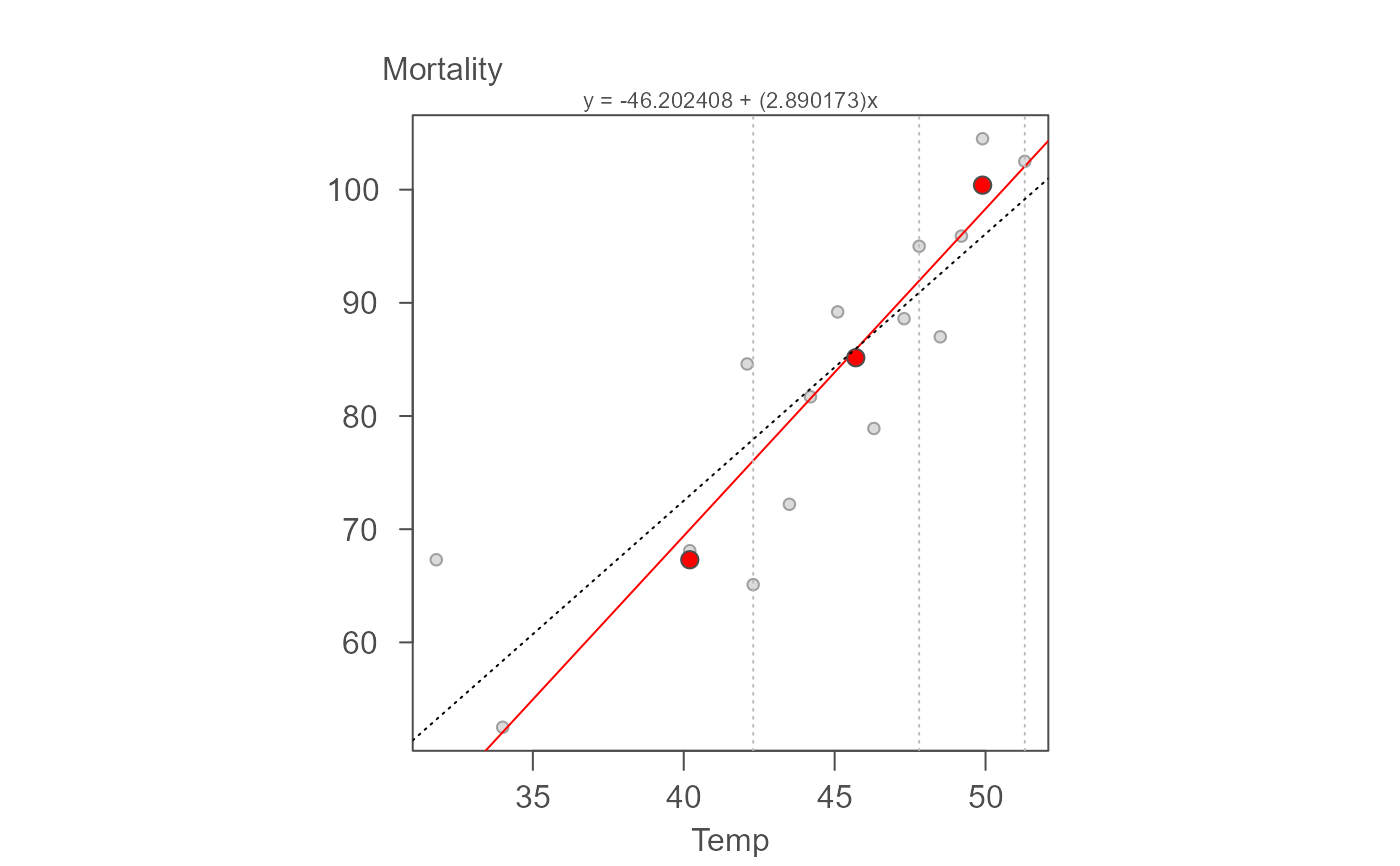 # Add a traditional OLS regression line (dashed blue line)
plot(M, reg = TRUE)
# Add a traditional OLS regression line (dashed blue line)
plot(M, reg = TRUE)
 #> int Temp^1
#> -21.794691 2.357695
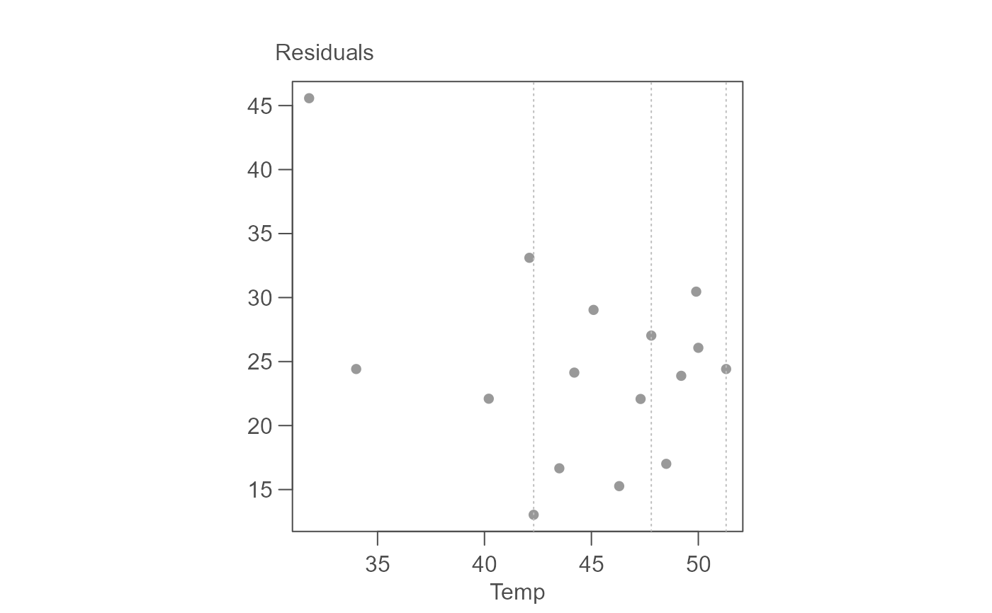
# Plot the residuals
plot(M, plot = "residuals")
#> int Temp^1
#> -21.794691 2.357695
# Plot the residuals
plot(M, plot = "residuals")
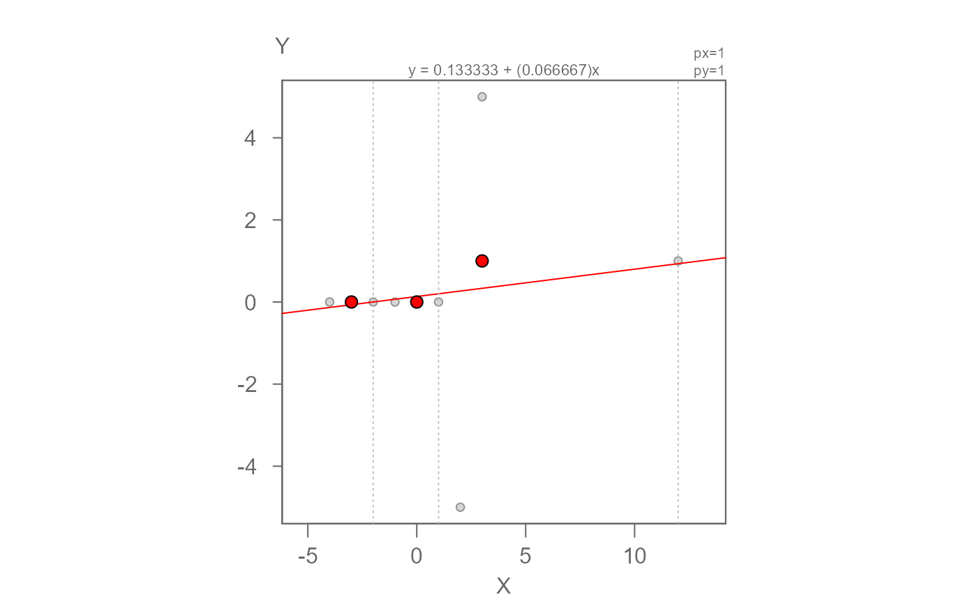
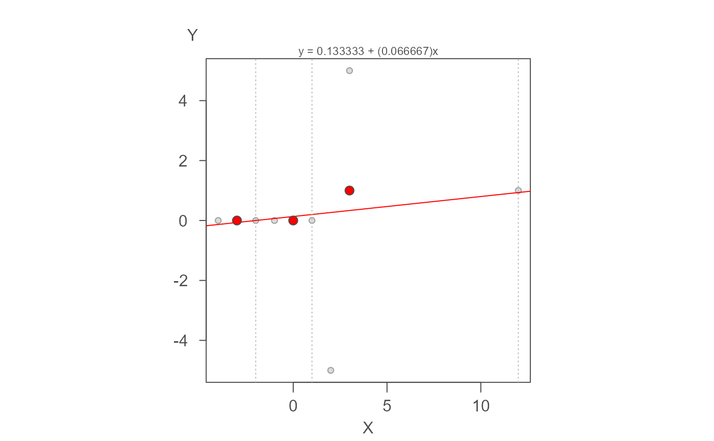 # This next example uses Andrew Siegel's pathological 9-point dataset to test
# for model stability when convergence cannot be reached.
M <- eda_rline(nine_point, X, Y)
plot(M)
# This next example uses Andrew Siegel's pathological 9-point dataset to test
# for model stability when convergence cannot be reached.
M <- eda_rline(nine_point, X, Y)
plot(M)