Multi-panel theoretical QQ plots

eda_theopan generates a multi-panel theoretical QQ plot for a continuous variable conditioned on a grouping variable.

Usage

eda_theopan(
  dat,
  x,
  fac,
  p = 1L,
  tukey = FALSE,
  base = exp(1),
  q.type = 5,
  dist = "norm",
  dist.l = list(),
  ylim = NULL,
  resid = FALSE,
  stat = mean,
  show.par = FALSE,
  plot = TRUE,
  grey = 0.6,
  pch = 21,
  nrow = 1,
  p.col = "grey40",
  p.fill = "grey60",
  size = 1,
  text.size = 0.8,
  tail.pch = 21,
  tail.p.col = "grey70",
  tail.p.fill = NULL,
  tic.size = 0.7,
  alpha = 0.8,
  q = FALSE,
  tails = FALSE,
  med = FALSE,
  inner = 0.75,
  iqr = TRUE,
  title = FALSE,
  xlab = NULL,
  ylab = NULL,
  ...
)

Arguments

dat: Data frame.
x: Continuous variable.
fac: Categorical variable.
p: Power transformation to apply to the continuous variable.
tukey: Boolean determining if a Tukey transformation should be adopted (FALSE adopts a Box-Cox transformation).
base: Base used with the log() function if p = 0.
q.type: An integer between 4 and 9 selecting one of the nine quantile algorithms. (See eda_fval for a list of quantile algorithms).
dist: Theoretical distribution to use. Defaults to Normal distribution.
dist.l: List of parameters passed to the distribution quantile function.
ylim: Y axes limits.
resid: Boolean determining if residuals should be plotted. Residuals are computed using the stat parameter.
stat: Statistic to use if residuals are to be computed. Currently mean (default) or median.
show.par: Boolean determining if power transformation should be displayed in the plot.
plot: Boolean determining if plot should be generated.
grey: Grey level to apply to plot elements (0 to 1 with 1 = black).
pch: Point symbol type.
nrow: Define the number of rows for panel layout.
p.col: Color for point symbol.
p.fill: Point fill color passed to bg (Only used for pch ranging from 21-25).
size: Point symbol size (0-1).
text.size: Size for category text above the plot.
tail.pch: Tail-end point symbol type (See tails).
tail.p.col: Tail-end color for point symbol (See tails).
tail.p.fill: Tail-end point fill color passed to bg (Only used for tail.pch ranging from 21-25).
tic.size: Size of tic labels (defaults to 0.8).
alpha: Point transparency (0 = transparent, 1 = opaque). Only applicable if rgb() is not used to define point colors.
q: Boolean determining if grey box highlighting the inner region should be displayed.
tails: Boolean determining if points outside of the inner region should be symbolized differently. Tail-end points are symbolized via the tail.pch, tail.p.col and tail.p.fill arguments.
med: Boolean determining if median lines should be drawn.
inner: Fraction of mid-values to highlight in q or tails. Defaults to the inner 75 percent of values.
iqr: Boolean determining if an IQR line should be fitted to the points.
title: Title to display. If set to TRUE, defaults to theoretical distribution type. If set to FALSE, omits title from output. Custom title can also be passed to this argument.
xlab: X-axis label.
ylab: Y-axis label.
...: Not used

Value

Returns a list with the following components:

data: List with input x and y values for each group. May be interpolated to smallest quantile batch if batch sizes don't match. Values will reflect power transformation defined in p

Details

The function will generate a multi-panel theoretical QQ plot. Currently, only the Normal QQ plot (dist="norm"), exponential QQ plot (dist="exp"), uniform QQ plot (dist="unif"), gamma QQ plot (dist="gamma"), chi-squared QQ plot (dist="chisq"), and the Weibull QQ plot (dist="weibull") are currently supported. By default, the Normal QQ plot maps the unit Normal quantiles to the x-axis (i.e. centered on a mean of 0 and standard deviation of 1 unit).

References

William S. Cleveland. Visualizing data. (1993)

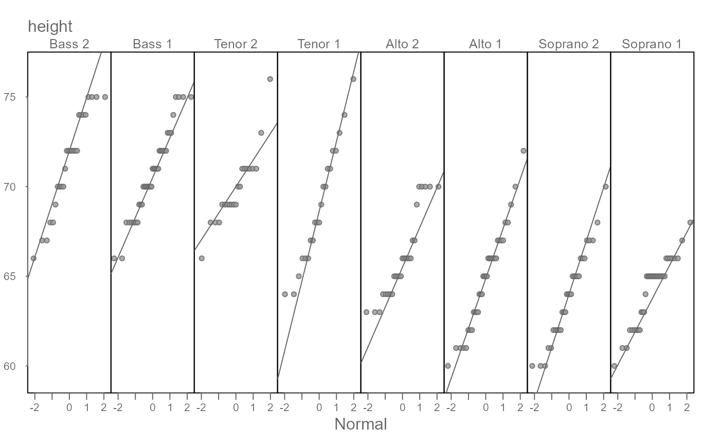
Examples


# Default output
singer <- lattice::singer
eda_theopan(singer, height, voice.part)


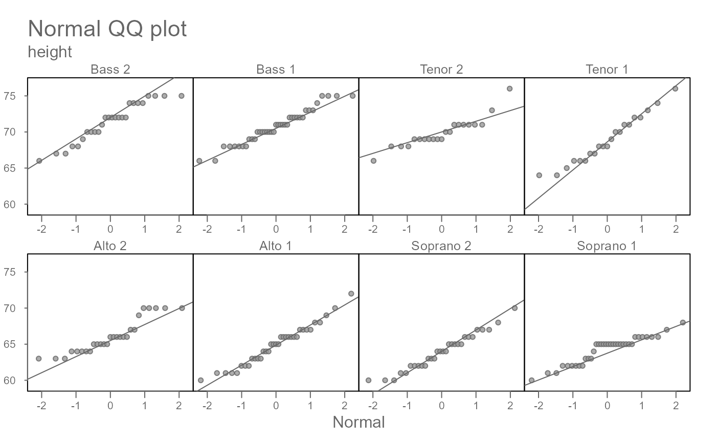
# Split into two rows
eda_theopan(singer, height, voice.part, nrow = 2, title = TRUE)


# Compare to a uniform distribution
eda_theopan(singer, height, voice.part, nrow = 2, dist = "unif")


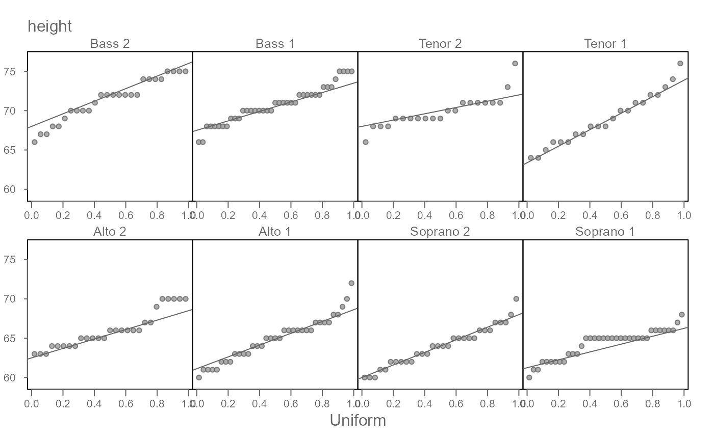# A uniform QQ plot is analogous to a Q(f) plot
eda_theopan(singer, height, voice.part, nrow = 2, dist = "unif",
              iqr = FALSE, xlab = "f-value")


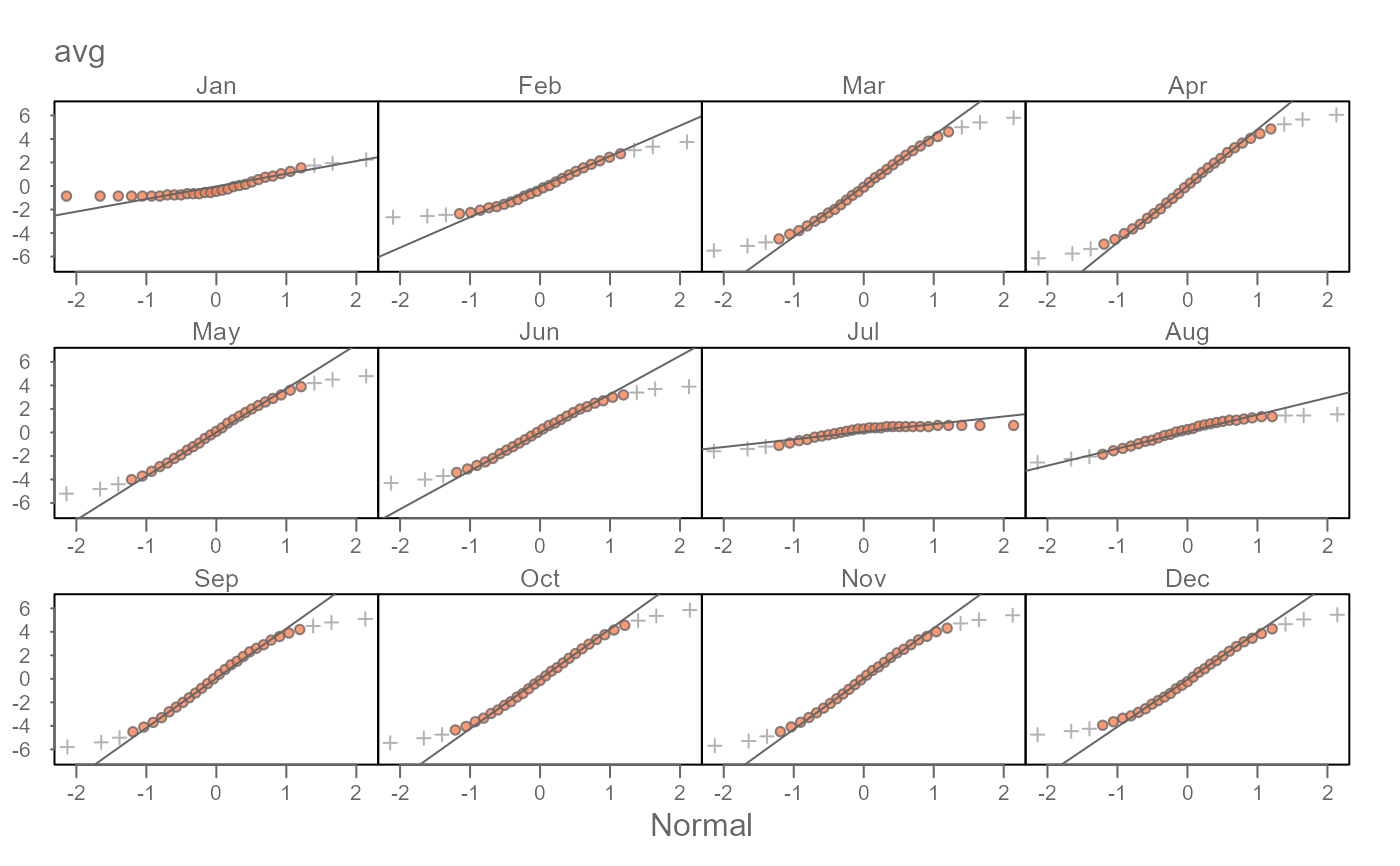
# Normal QQ plots of Waterville daily averages. Mean monthly values are
# subtracted from the data to recenter all batches around 0.  Color and point
# symbols are used to emphasize the inner core of the data (here set to the
# inner 80% of values)
wat <- tukeyedar::wat05
wat$month <- factor(format(wat$date,"%b"), levels = month.abb)
eda_theopan(wat,avg, month, resid = TRUE, nrow = 3, inner = 0.8 ,
                    tails = TRUE, tail.pch = 3, p.fill = "coral")