Plot method for eda_mean_sweep objects — plot.eda_mean

Generates decomposition plots or diagnostic plots from an object of class "eda_mean_sweep".

Usage

# S3 method for class 'eda_mean_sweep'
plot(
  x,
  plot = "effects",
  reg = TRUE,
  margin = NULL,
  legend = TRUE,
  legend.pos = "bottomright",
  legend.inset = 0.03,
  ...
)

Arguments

x

An object of class eda_mean_sweep

plot

A character string specifying the type of plot.

"effects": (default) Plots the raw centered effects.
"ms": Scales effects by sqrt(N / df) to reflect their relative contribution to variance.
"diagnostic": Generates a diagnostic plot of residuals versus comparison values to check for non-additivity (interactions). This is typically used on a model with main effects only.

reg

Logical. If TRUE (the default), fits a linear regression line to the diagnostic plot. This is disabled when margin = "all".

margin

Character string. Only used when plot = "diagnostic". Specifies which interaction to diagnose. Can be the name of a two-way interaction (e.g., "FactorA:FactorB") or "all" (the default) to overlay diagnostics for all two-way interactions.

legend

Logical. If TRUE, a legend is added when margin = "all".

legend.pos

The position of the legend, e.g., "bottomright".

legend.inset

The amount of inset for the legend from the plot border.

...

Additional arguments passed to the internal plotting function. See .eda_plot_vardecomp for the "effects" plot or .eda_plot_xy for the "diagnostic" plot (e.g., loe, sd).

Value

A plot visualizing residuals and factor effects.

Details

This plot method can generate two types of plots:

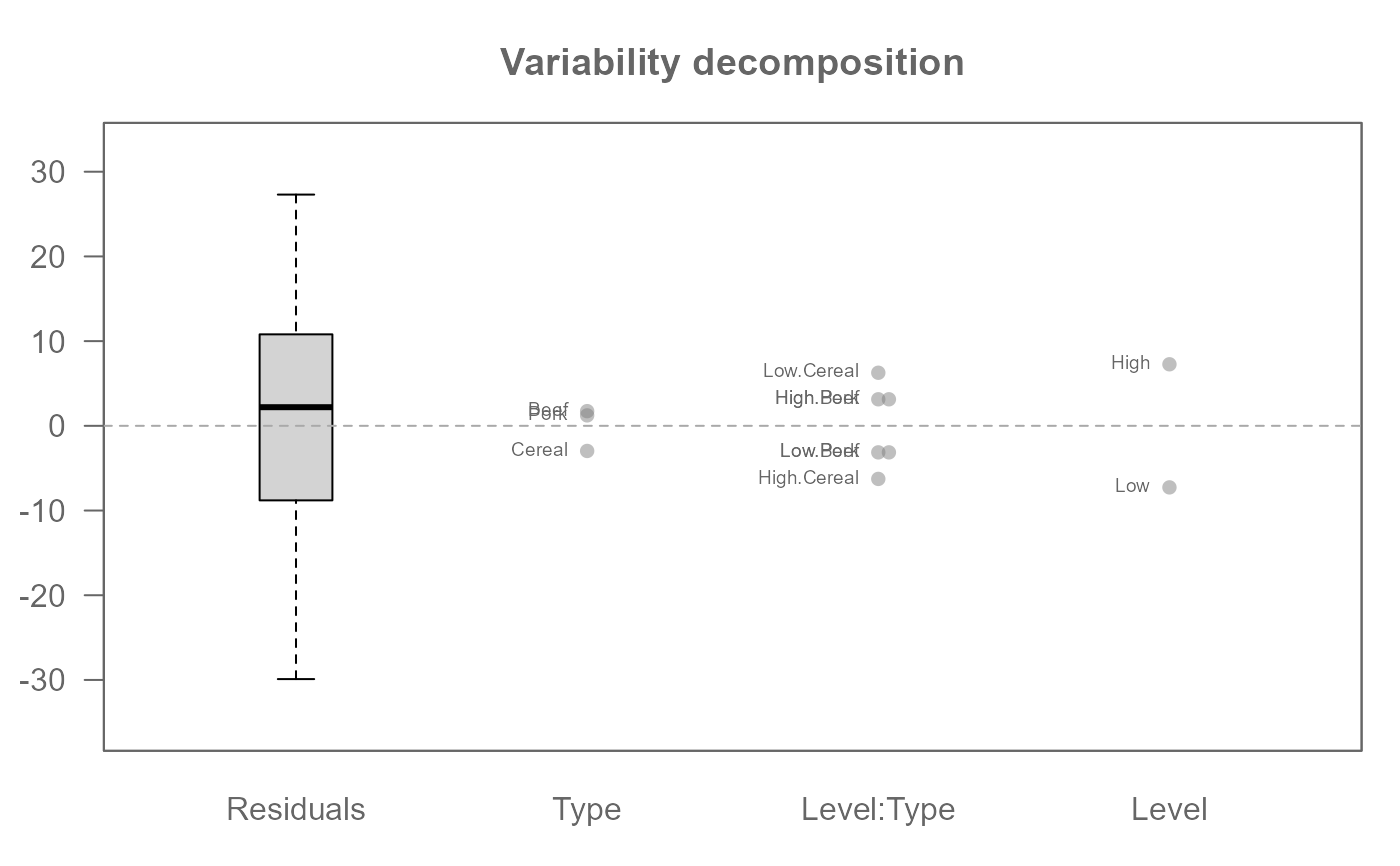
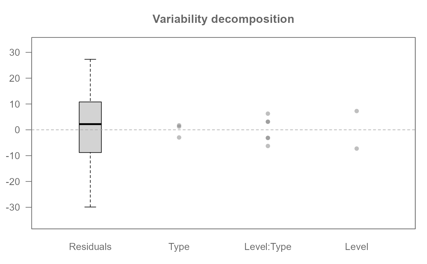
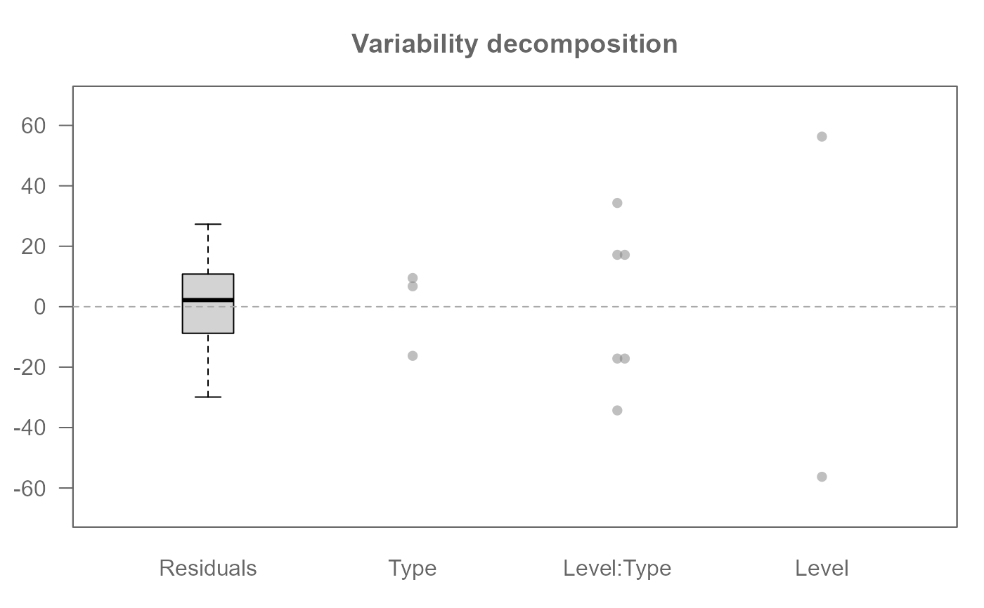
1. Variability Decomposition Plot (plot = "effects" or "ms")
This plot, handled by .eda_plot_vardecomp, visualizes the additive overlays: the residuals and the centered main and interaction effects.

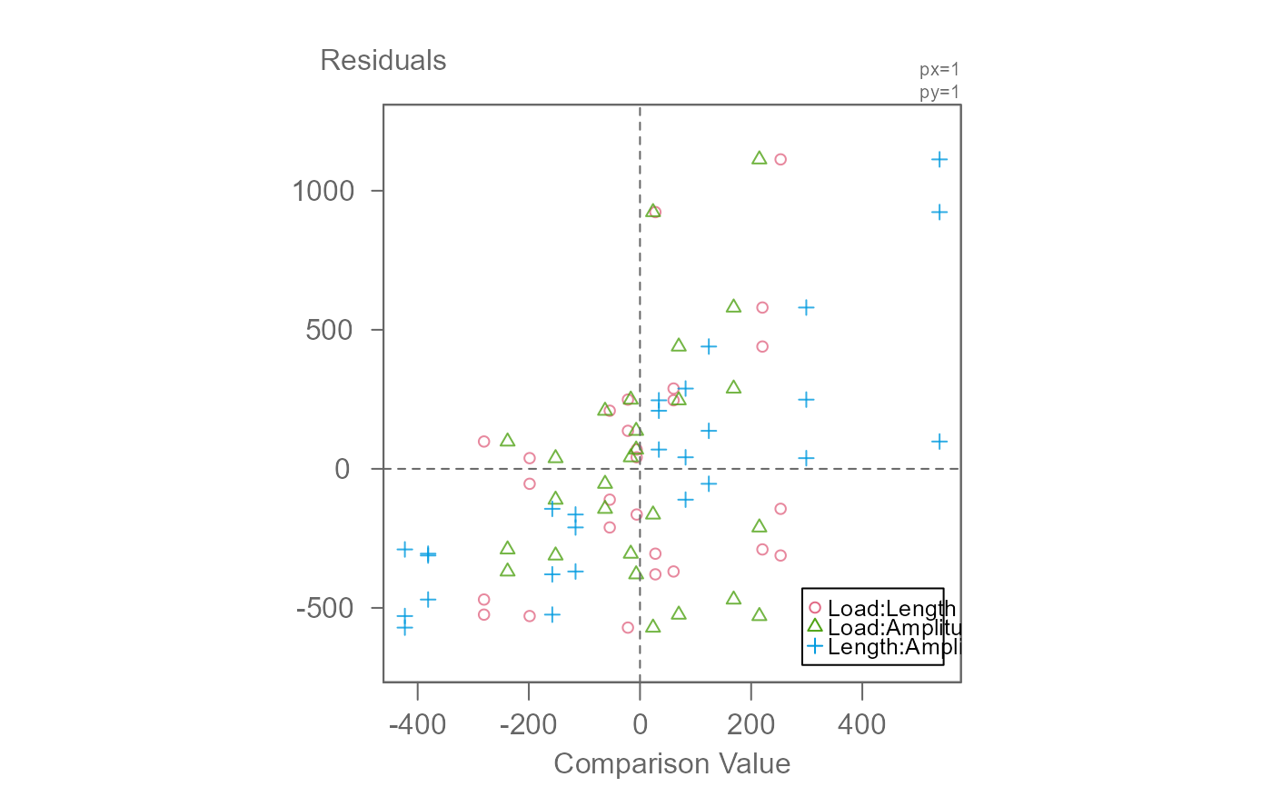
2. Diagnostic Plot (plot = "diagnostic")
This plot is a key tool from Exploratory Data Analysis for assessing if an additive model is sufficient. It plots the residuals from the model against a set of "comparison values". For a two-way model, the comparison value is:
(row effect) * (column effect) / (grand mean)
A sloping trend in this plot suggests a hidden interaction.

References

Hoaglin, D. C., Mosteller, F., & Tukey, J. W. (1991). Fundamentals of Exploratory Analysis of Variance. Wiley.

Examples


# A default plot
M0 <- eda_mean_sweep(feav5_12, Weight, Level, Type, max_order = 2)
plot(M0)


# Adding labels
plot(M0, label = TRUE)


# Options are available for dot plots when tes are present. By default, points
# are stacked. Other options include "jitter",
plot(M0, overlap = "jitter")


# ... or "overplot" (you can modify the point transparency via the "alpha" argument)
plot(M0, overlap = "overplot")


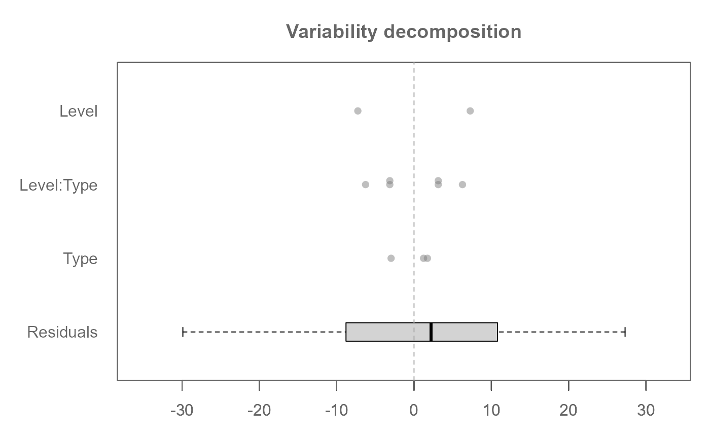
# Plot can be rotated
plot(M0, rotate = TRUE)


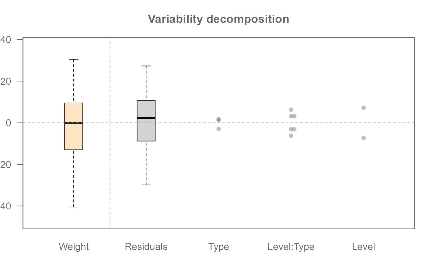
# Original response variable can be added as a boxplot
plot(M0, show.resp = TRUE)


# If "mean squares" are to be compared, the effects need to be adjusted
# by setting plot = "ms" (see page 174 of the referenced source)
plot(M0, plot = "ms")


# Generating diagnostic plots
M1 <- eda_mean_sweep(yarn, Cycles, Load, Length, Amplitude)

# Create an overlay of all two-way diagnostic plots
# Note: For mean-sweep, this plots Residuals vs. CV for each interaction
plot(M1, plot = "diagnostic", margin = "all")
#> For 'margin = "all"', regression lines are disabled to avoid confusion.


# Create a diagnostic plot for a specific interaction
plot(M1, plot = "diagnostic", margin = "Load:Length", reg = TRUE)

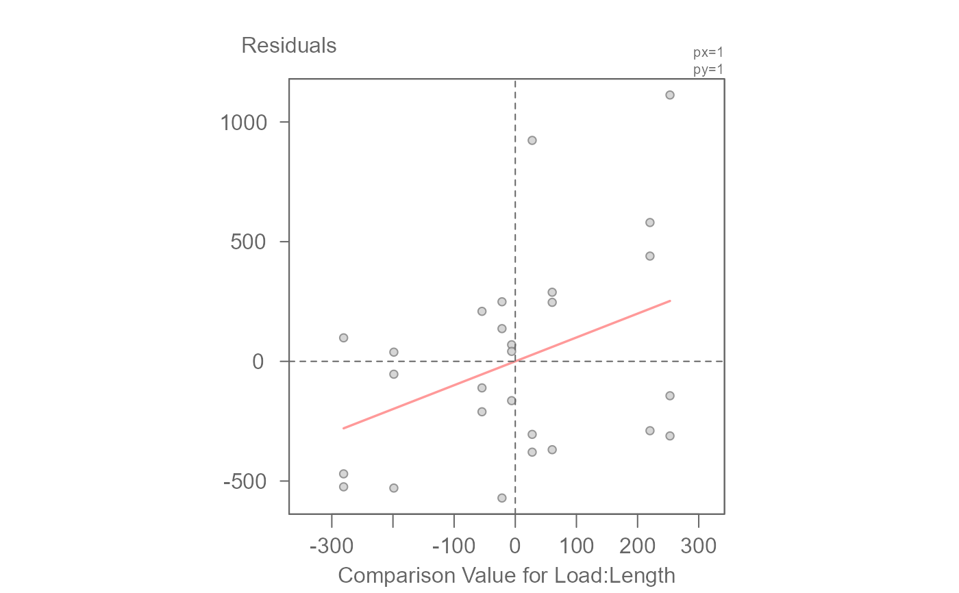#>                                int Comparison Value for Load:Length^1 
#>                      -6.018285e-14                       9.971699e-01

Plot method for `eda_mean_sweep` objects