Chapter 10 Map Algebra
10.1 Introduction
Cartographic modeling is a structured approach to geographic analysis that uses a language of operations to interpret spatial data. These operations are organized into functional categories that describe how data values are transformed and combined across geographic space. The modeling system, as developed by Dana Tomlin (Tomlin 1990) is built around three core spatial contexts:
Local operations: Compute new values for each location based on data explicitly associated with that location, often across one or more layers.
Focal operations: Compute values based on the surrounding neighborhood of each location. These neighborhoods can be defined by distance, direction, travel cost, or visibility.
Zonal operations: Aggregate data across defined zones, which are mutually exclusive and collectively exhaustive areas of the study region.
In addition to these, O’Sullivan and Unwin (O’Sullivan and Unwin 2010) propose a fourth category: global operations. These refer to analytical functions that consider all locations in a dataset simultaneously, such as calculating overall statistics, evaluating spatial autocorrelation, or computing Euclidean distances to nearest features.
10.2 Local operations and functions
Local operations are the most fundamental type of cartographic modeling function. They compute a new value for each location based solely on the data explicitly associated with that same location—either from a single layer or from multiple layers.
For instance, starting with an original raster layer, we might apply a sequence of operations—first multiplying each cell value by 2, then adding 1. The result is a new raster in which each cell reflects the cumulative effect of those operations applied to the corresponding cell in the original layer. This is an example of a unary operation, where only a single raster is involved in the computation.
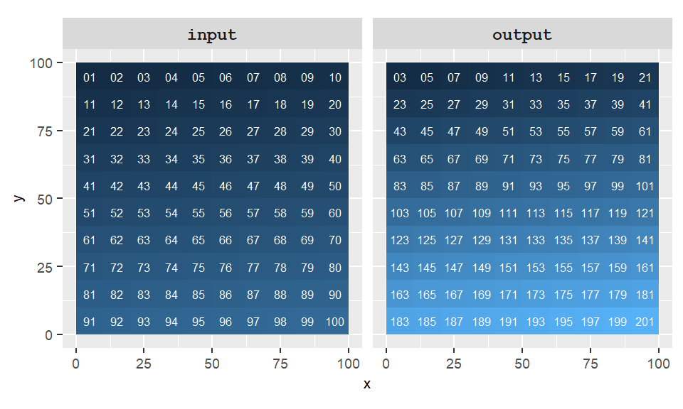
Figure 10.1: Example of a local operation where output=(2 * raster + 1).
Local operations can also involve multiple raster layers. For example, two rasters can be added together by summing the values of overlapping cells, resulting in a new raster where each cell reflects the combined value from the corresponding cells in the input layers.
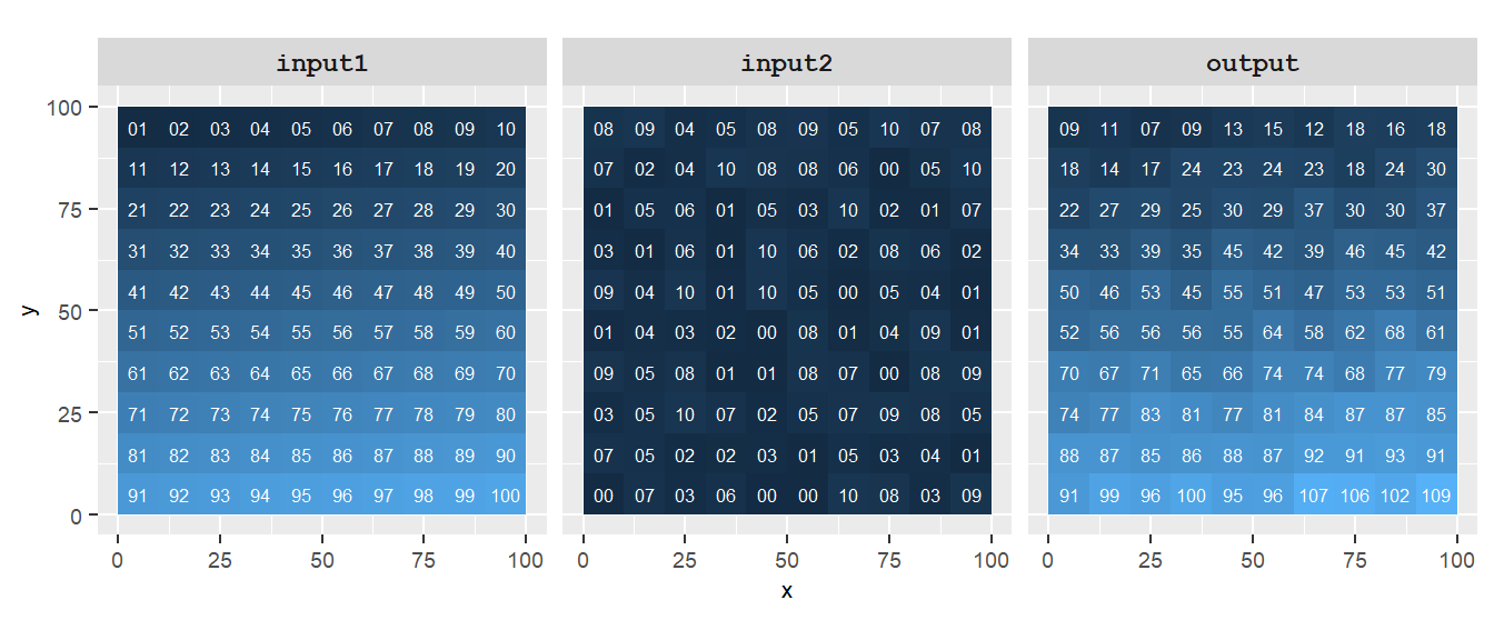
Figure 10.2: Example of a local operation where output=(input1+input2). Note how each cell output only involves input raster cells that share the same exact location.
Local operations also include reclassification, where a range of input raster values is assigned a new, common value. This technique is useful for grouping data into meaningful categories. For example, we might reclassify the input raster values as follows:
| Original values | Reclassified values |
|---|---|
| 0-25 | 25 |
| 26-50 | 50 |
| 51-75 | 75 |
| 76-100 | 100 |
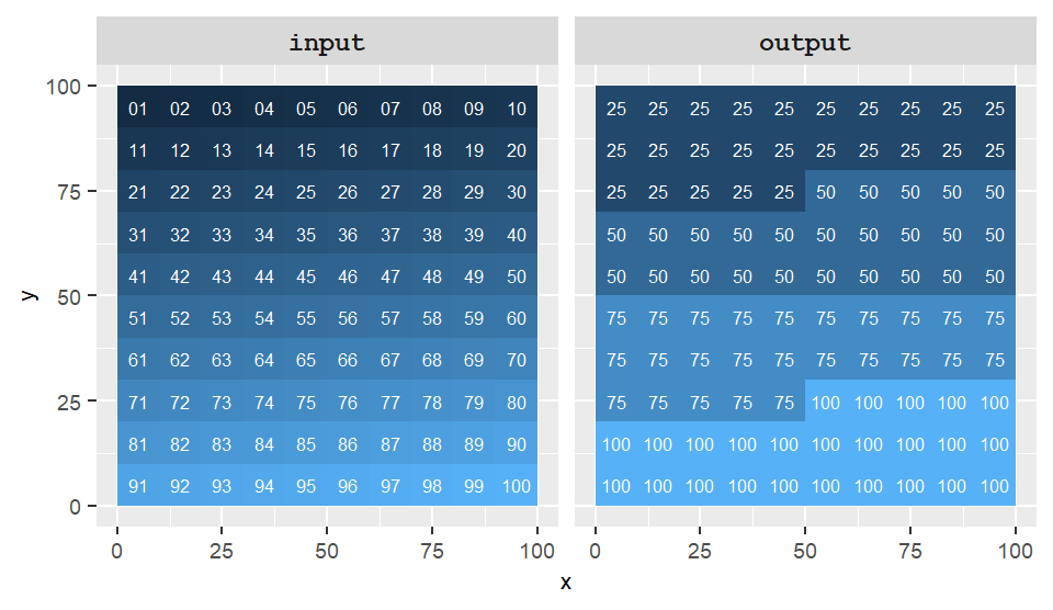
Figure 10.3: Example of a local operation where the output results from the reclassification of input values.
10.3 Focal operations and functions
Focal operations differ from local operations in that they consider the values of neighboring cells when computing a new value for each location. Instead of looking only at a single cell, focal functions examine a defined neighborhood–such as the eight adjacent cells surrounding a central location.
For example, a focal operation might calculate the average of all neighboring cell values and assign that average to the central cell. This approach is useful for smoothing data, detecting spatial patterns, and identifying transitions across a surface.
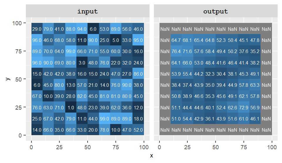
Figure 10.4: Example of a focal operation where the output cell values take on the average value of neighboring cells from the input raster. Focal cells surrounded by non-existent cells are assigned an NA in this example.
Notice in the example above that the edge cells in the output raster have been assigned a value of NA (No Data). This occurs because the neighborhood around those edge cells extends beyond the raster’s boundary, where no values exist. Some GIS applications handle this differently—they may ignore the missing surrounding cells and compute the average using only the available neighboring values, as demonstrated in the next example.
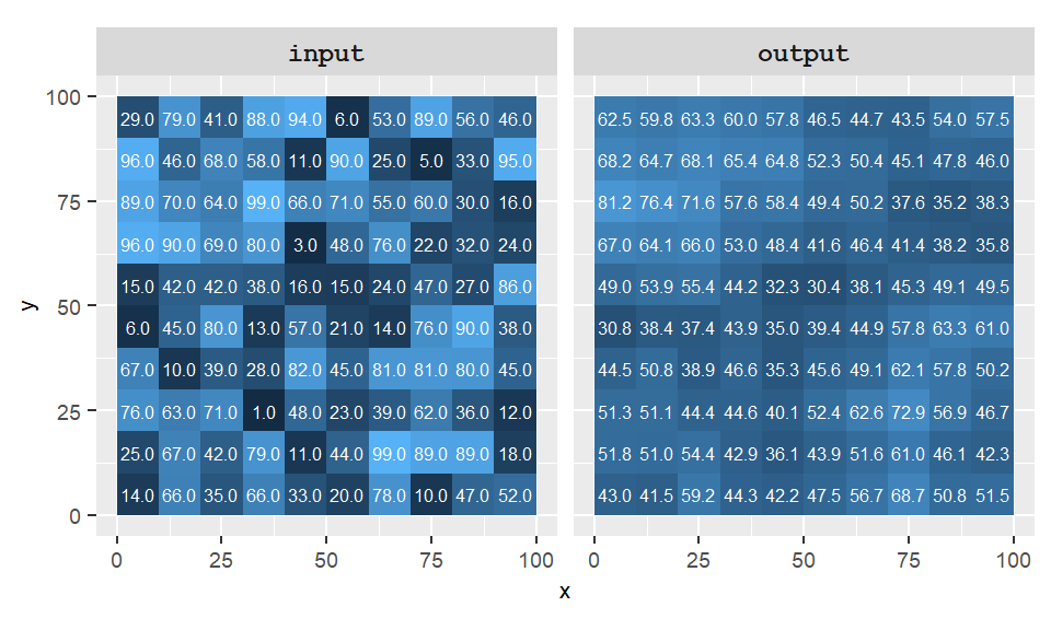
Figure 10.5: Example of a focal operation where the output cell values take on the average value of neighboring cells from the input raster. Surrounding non-existent cells are ignored.
Focal (or neighborhood) operations require the definition of a window region, commonly referred to as a kernel. In the examples above, a simple 3×3 kernel was used, where each cell’s value was influenced by its immediate neighbors. The kernel itself can vary in both size and shape—for instance, a 3×3 square where the central cell is excluded (resulting in eight neighbors), or a circular neighborhood defined by a specified radius.
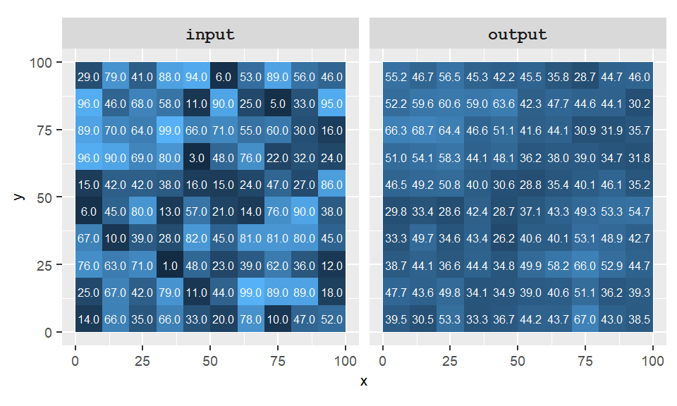
Figure 10.6: Example of a focal operation where the kernel is defined by a 3 by 3 cell without the center cell, and whose output cell takes on the average value of those neighboring cells.
n addition to defining the shape and size of the neighborhood, a kernel also specifies the weight each neighboring cell contributes to the summary statistic. For example, in a 3×3 neighborhood, each cell might contribute an equal weight of 1/9th to the final value. However, weights can also be defined using more complex functions–these are known as kernel functions. One commonly used kernel function is the Gaussian, which assigns greater weight to cells closer to the center and less to those farther away.
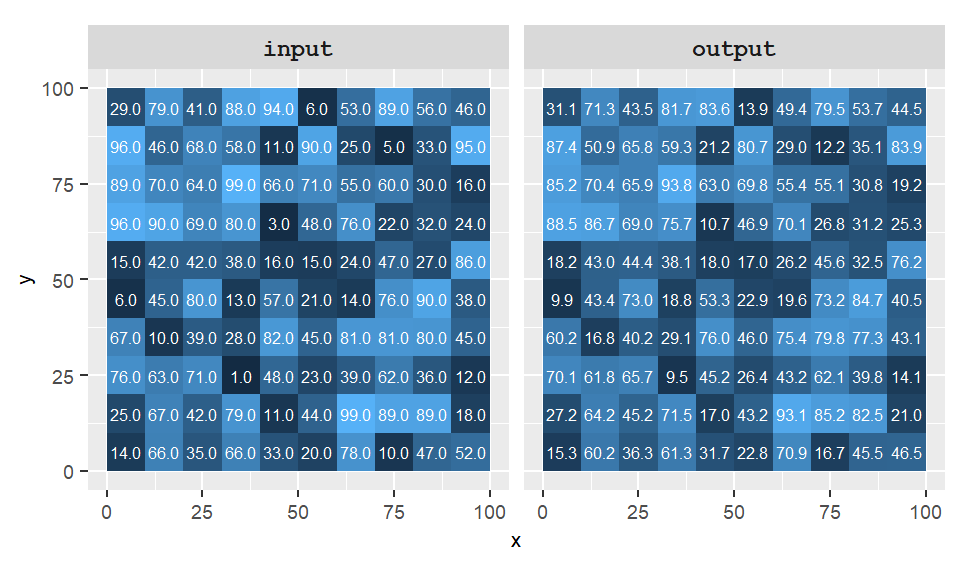
Figure 10.7: Example of a focal operation where the kernel is defined by a Gaussian function whereby the closest cells are assigned a greater weight.
10.4 Zonal operations and functions
Zonal operations differ from local and focal operations in that they summarize values across defined zones rather than individual cells or neighborhoods. A zone is a group of cells that share a common value on a separate raster layer—often representing administrative boundaries, land parcels, or other categorical regions.
In the following example, the cell values from the raster layer are aggregated into three zones whose boundaries are delineated by red polygons. Each output zone shows the average value of the cells within that zone.
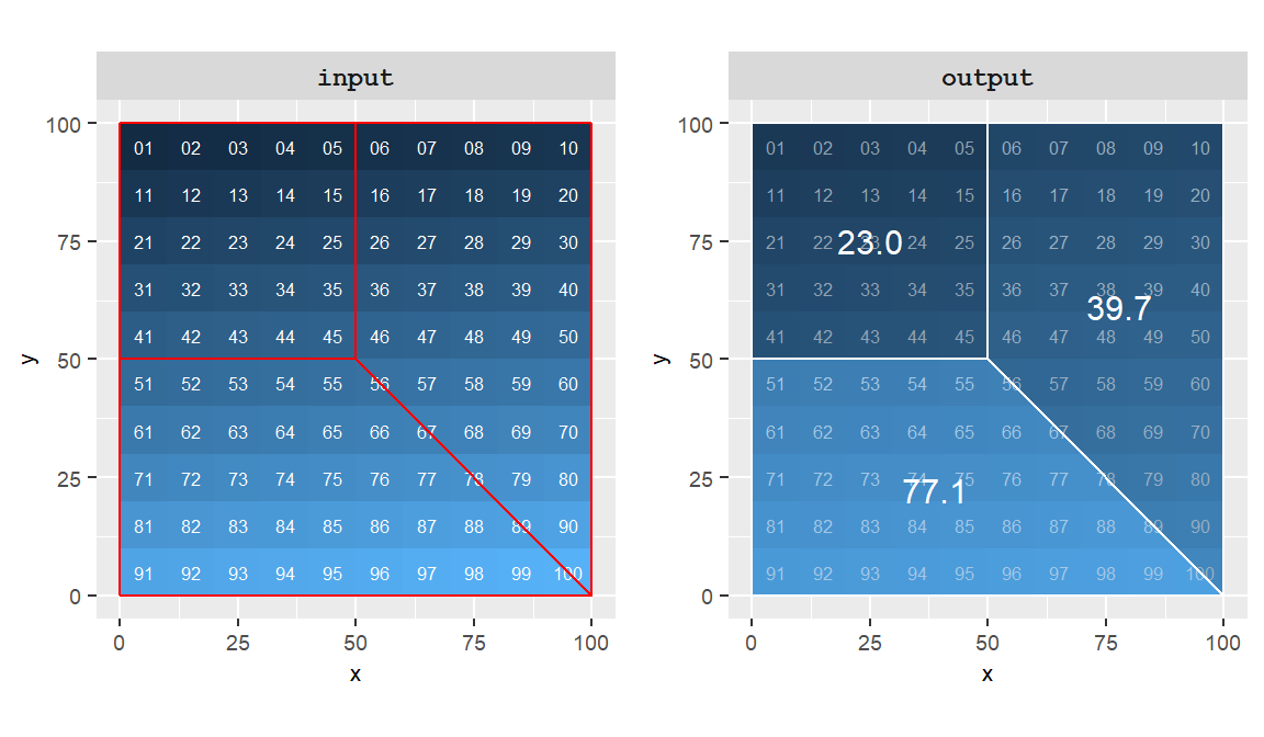
Figure 10.8: Example of a zonal operation where the cell values are averaged for each of the three zones delineated in red.
While rasters can be used to define zones, it’s more common for a GIS to have a polygon layer define the zones.
10.5 Global operations and functions
Global operations and functions may use some or all input cells when computing the value of each output cell. A common example is the Euclidean Distance tool, which calculates the shortest straight-line distance between each cell and a specified source or destination. In the example below, a new raster assigns to each cell the distance to the nearest cell with a value of 1–note that only two such cells exist in the input raster.
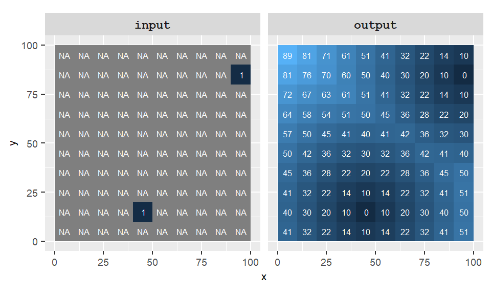
Figure 10.9: Example of a global function: the Euclidean distance. Each pixel is assigned its closest distance to one of the two source locations (defined in the input layer).
Global operations and functions can also generate single value outputs such as the overall pixel mean or standard deviation.
Another popular use of global functions is in the mapping of least-cost paths where a cost surface raster is used to identify the shortest path between two locations which minimizes cost (in time or money).
10.6 Operators and functions
Operations and functions applied to gridded data can be broken down into three groups: mathematical, logical comparison and Boolean.
10.6.1 Mathematical operators and functions
Two mathematical operators have already been demonstrated in earlier sections: the multiplier and the addition operators. Other operators include division and the modulo (also known as the modulus) which is the remainder of a division. Mathematical functions can also be applied to gridded data manipulation. Examples are square root and sine functions. The following table showcases a few examples with ArcGIS and R syntax.
| Operation | ArcGIS Syntax | R Syntax | Example |
|---|---|---|---|
| Addition | + |
+ |
input1 + input2 |
| Subtraction | - |
- |
input1 - input2 |
| Division | / |
/ |
input1 / input2 |
| Modulo | Mod() |
%% |
Mod(input1, 100), input1 %% 10 |
| Square root | SquareRoot() |
sqrt() |
SquareRoot(input1), sqrt(input1) |
10.6.2 Logical comparison
The logical comparison operators evaluate a condition then output a value of 1 if the condition is true and 0 if the condition is false. Logical comparison operators consist of greater than, less than, equal and not equal.
| Logical comparison | Syntax |
|---|---|
| Greater than | > |
| Less than | < |
| Equal | == |
| Not equal | != |
For example, the following figure shows the output of the comparison between two rasters where we are assessing if cells in input1 are greater than those in input2 (on a cell-by-cell basis).
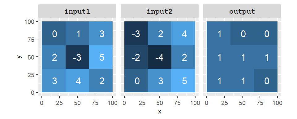
Figure 10.10: Output of the operation input1 > input2. A value of 1 in the output raster indicates that the condition is true and a value of 0 indicates that the condition is false.
When assessing whether two cells are equal, some programming environments such as R and ArcGIS’s Raster Calculator require the use of the double equality syntax, ==, as in input1 == input2. In these programming environments, the single equality syntax is usually interpreted as an assignment operator so input1 = input2 would instruct the computer to assign the cell values in input2 to input1 (which is not what we want to do here).
Some applications make use of special functions to test a condition. For example, ArcGIS has a function called Con(condition, out1, out2) which assigns the value out1 if the condition is met and a value of out2 if it’s not. For example, ArcGIS’s raster calculator expression
Con( input1 > input2, 1, 0)outputs a value of 1 if input1 is greater than input2 and 0 if not. It generates the same output as the one shown in the above figure. Note that in most programming environments (including ArcGIS), the expression input1 > input2 produces the same output because the value 1 is the numeric representation of TRUE and 0 that of FALSE.
10.6.3 Boolean (or Logical) operators
In map algebra, Boolean operators are used to compare conditional states of a cell (i.e. TRUE or FALSE). The three Boolean operators are AND, OR and NOT.
| Boolean | ArcGIS | R | Example |
|---|---|---|---|
| AND | & | & | input1 & input2 |
| OR | | |
| |
input1 | input2 |
| NOT | ~ |
! |
~input2, ! input2 |
A “TRUE” state is usually encoded as a
1or any non-zero integer while a “FALSE” state is usually encoded as a0.
For example, if cell1=0 and cell2=1, the Boolean operation cell1 AND cell2 results in a FALSE (or 0) output cell value. This Boolean operation can be translated into plain English as “are the cells 1 and 2 both TRUE?” to which we answer “No they are not” (cell1 is FALSE). The OR operator can be interpreted as “is x or y TRUE?” so that cell1 OR cell2 would return TRUE. The NOT interpreter can be interpreted as “is x not TRUE?” so that NOT cell1 would return TRUE.
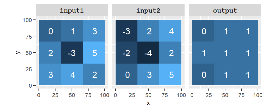
Figure 10.11: Output of the operation input1 AND input2. A value of 1 in the output raster indicates that the condition is true and a value of 0 indicates that the condition is false. Note that many programming environments treat any none 0 values as TRUE so that -3 AND -4 will return TRUE.
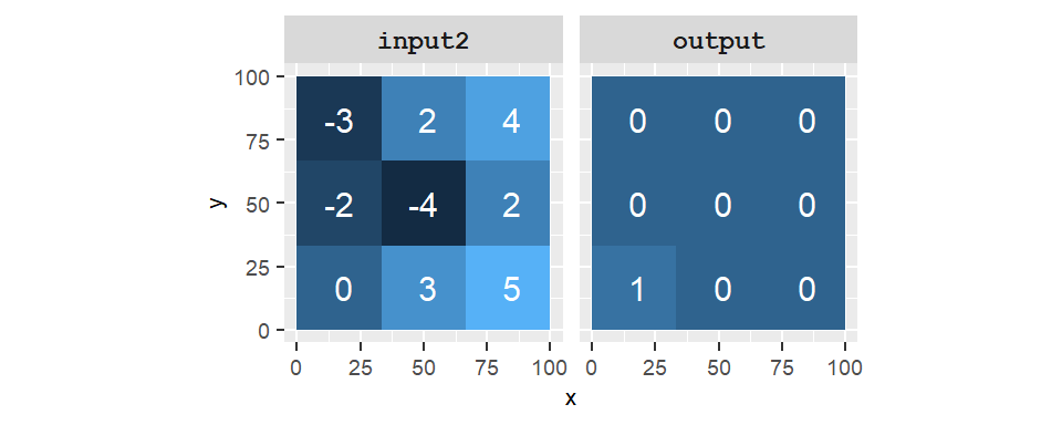
Figure 10.12: Output of the operation NOT input2. A value of 1 in the output raster indicates that the input cell is NOT TRUE (i.e. has a value of 0).
10.6.4 Combining operations
Both comparison and Boolean operations can be combined into a single expression. For example, we may wish to find locations (cells) that satisfy requirements from two different raster layers: e.g. 0<input1<4 AND input2>0. To satisfy the first requirement, we can write out the expression as (input1>0) & (input1<4). Both comparisons (delimited by parentheses) return a 0 (FALSE) or a 1 (TRUE). The ampersand, &, is a Boolean operator that checks that both conditions are met and returns a 1 if yes or a 0 if not. This expression is then combined with another comparison using another ampersand operator that assesses the criterion input2>0. The amalgamated expression is thus ((input1>0) & (input1<4)) & (input2>0).
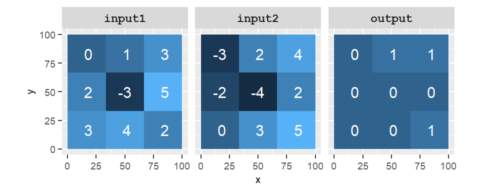
Figure 10.13: Output of the operation ((input1>0) & (input1<4)) & (input2>0). A value of 1 in the output raster indicates that the condition is true and a value of 0 indicates that the condition is false.
Note that most software environments assign the ampersand character,
&, to theANDBoolean operator.
10.7 Summary
In this chapter, we explored the foundational concepts of Map Algebra, a framework for performing spatial analysis using raster data. We examined how local, focal, zonal, and global operations each contribute to different types of spatial reasoning. Local operations focus on individual cells, focal operations incorporate neighborhood context, zonal operations summarize values across defined regions, and global operations consider the entire raster dataset.