G Coordinate Systems in R

R	terra	sf	tmap	geosphere
4.4.0	1.7.78	1.0.16	3.3.4	1.5.18

A note about the changes to the PROJ environment

Newer versions of sf make use of the PROJ 6.0 C library or greater. Note that the version of PROJ is not to be confused with the version of the proj4 R package–the proj4 and sf packages make use of the PROJ C library that is developed independent of R. You can learn more about the PROJ development at proj.org.

There has been a significant change in the PROJ library since the introduction of version 6.0. This has had serious implications in the development of the R spatial ecosystem. As such, if you are using an older version of sf or proj4 that was developed with a version of PROJ older than 6.0, some of the input/output presented in this appendix may differ from yours.

Sample files for this exercise

Data used in this exercise can be loaded into your current R session by running the following chunk of code.

library(terra)

z <- gzcon(url("https://github.com/mgimond/Spatial/raw/main/Data/elev.RDS"))
elev.r <- unwrap(readRDS(z))
z <- gzcon(url("https://github.com/mgimond/Spatial/raw/main/Data/s_sf.RDS"))
s.sf <- readRDS(z)

We’ll make use of two data layers in this exercise: a Maine counties polygon layer (s.sf) and an elevation raster layer (elev.r). The former is in an sf format and the latter is in a SpatRaster format.

Loading the sf package

library(sf)   

Note the versions of GEOS, GDAL and PROJ the package sf is linked to. Different versions of these libraries may result in different outcomes than those shown in this appendix. You can check the linked library versions as follows:

sf_extSoftVersion()[1:3]

    GEOS     GDAL   proj.4 
"3.12.1"  "3.8.4"  "9.3.1" 

Checking for a coordinate system

To extract coordinate system (CS) information from an sf object use the st_crs function.

st_crs(s.sf)

Coordinate Reference System:
  User input: EPSG:26919 
  wkt:
PROJCRS["NAD83 / UTM zone 19N",
    BASEGEOGCRS["NAD83",
        DATUM["North American Datum 1983",
            ELLIPSOID["GRS 1980",6378137,298.257222101,
                LENGTHUNIT["metre",1]]],
        PRIMEM["Greenwich",0,
            ANGLEUNIT["degree",0.0174532925199433]],
        ID["EPSG",4269]],
    CONVERSION["UTM zone 19N",
        METHOD["Transverse Mercator",
            ID["EPSG",9807]],
        PARAMETER["Latitude of natural origin",0,
            ANGLEUNIT["degree",0.0174532925199433],
            ID["EPSG",8801]],
        PARAMETER["Longitude of natural origin",-69,
            ANGLEUNIT["degree",0.0174532925199433],
            ID["EPSG",8802]],
        PARAMETER["Scale factor at natural origin",0.9996,
            SCALEUNIT["unity",1],
            ID["EPSG",8805]],
        PARAMETER["False easting",500000,
            LENGTHUNIT["metre",1],
            ID["EPSG",8806]],
        PARAMETER["False northing",0,
            LENGTHUNIT["metre",1],
            ID["EPSG",8807]]],
    CS[Cartesian,2],
        AXIS["(E)",east,
            ORDER[1],
            LENGTHUNIT["metre",1]],
        AXIS["(N)",north,
            ORDER[2],
            LENGTHUNIT["metre",1]],
    USAGE[
        SCOPE["Engineering survey, topographic mapping."],
        AREA["North America - between 72°W and 66°W - onshore and offshore. Canada - Labrador; New Brunswick; Nova Scotia; Nunavut; Quebec. Puerto Rico. United States (USA) - Connecticut; Maine; Massachusetts; New Hampshire; New York (Long Island); Rhode Island; Vermont."],
        BBOX[14.92,-72,84,-66]],
    ID["EPSG",26919]]

With the newer version of the PROJ C library, the coordinate system is defined using the Well Known Text (WTK/WTK2) format which consists of a series of [...] tags. The WKT format will usually start with a PROJCRS[...] tag for a projected coordinate system, or a GEOGCRS[...] tag for a geographic coordinate system.

The CRS output will also consist of a user defined CS definition which can be an EPSG code (as is the case in this example), or a string defining the datum and projection type.

You can also extract CS information from a SpatRaster object use the st_crs function.

st_crs(elev.r)

Coordinate Reference System:
  User input: BOUNDCRS[
    SOURCECRS[
        PROJCRS["unknown",
            BASEGEOGCRS["unknown",
                DATUM["North American Datum 1983",
                    ELLIPSOID["GRS 1980",6378137,298.257222101,
                        LENGTHUNIT["metre",1]],
                    ID["EPSG",6269]],
                PRIMEM["Greenwich",0,
                    ANGLEUNIT["degree",0.0174532925199433],
                    ID["EPSG",8901]]],
            CONVERSION["UTM zone 19N",
                METHOD["Transverse Mercator",
                    ID["EPSG",9807]],
                PARAMETER["Latitude of natural origin",0,
                    ANGLEUNIT["degree",0.0174532925199433],
                    ID["EPSG",8801]],
                PARAMETER["Longitude of natural origin",-69,
                    ANGLEUNIT["degree",0.0174532925199433],
                    ID["EPSG",8802]],
                PARAMETER["Scale factor at natural origin",0.9996,
                    SCALEUNIT["unity",1],
                    ID["EPSG",8805]],
                PARAMETER["False easting",500000,
                    LENGTHUNIT["metre",1],
                    ID["EPSG",8806]],
                PARAMETER["False northing",0,
                    LENGTHUNIT["metre",1],
                    ID["EPSG",8807]],
                ID["EPSG",16019]],
            CS[Cartesian,2],
                AXIS["(E)",east,
                    ORDER[1],
                    LENGTHUNIT["metre",1,
                        ID["EPSG",9001]]],
                AXIS["(N)",north,
                    ORDER[2],
                    LENGTHUNIT["metre",1,
                        ID["EPSG",9001]]]]],
    TARGETCRS[
        GEOGCRS["WGS 84",
            DATUM["World Geodetic System 1984",
                ELLIPSOID["WGS 84",6378137,298.257223563,
                    LENGTHUNIT["metre",1]]],
            PRIMEM["Greenwich",0,
                ANGLEUNIT["degree",0.0174532925199433]],
            CS[ellipsoidal,2],
                AXIS["geodetic latitude (Lat)",north,
                    ORDER[1],
                    ANGLEUNIT["degree",0.0174532925199433]],
                AXIS["geodetic longitude (Lon)",east,
                    ORDER[2],
                    ANGLEUNIT["degree",0.0174532925199433]],
            ID["EPSG",4326]]],
    ABRIDGEDTRANSFORMATION["Transformation from unknown to WGS84",
        METHOD["Geocentric translations (geog2D domain)",
            ID["EPSG",9603]],
        PARAMETER["X-axis translation",0,
            ID["EPSG",8605]],
        PARAMETER["Y-axis translation",0,
            ID["EPSG",8606]],
        PARAMETER["Z-axis translation",0,
            ID["EPSG",8607]]]] 
  wkt:
BOUNDCRS[
    SOURCECRS[
        PROJCRS["unknown",
            BASEGEOGCRS["unknown",
                DATUM["North American Datum 1983",
                    ELLIPSOID["GRS 1980",6378137,298.257222101,
                        LENGTHUNIT["metre",1]],
                    ID["EPSG",6269]],
                PRIMEM["Greenwich",0,
                    ANGLEUNIT["degree",0.0174532925199433],
                    ID["EPSG",8901]]],
            CONVERSION["UTM zone 19N",
                METHOD["Transverse Mercator",
                    ID["EPSG",9807]],
                PARAMETER["Latitude of natural origin",0,
                    ANGLEUNIT["degree",0.0174532925199433],
                    ID["EPSG",8801]],
                PARAMETER["Longitude of natural origin",-69,
                    ANGLEUNIT["degree",0.0174532925199433],
                    ID["EPSG",8802]],
                PARAMETER["Scale factor at natural origin",0.9996,
                    SCALEUNIT["unity",1],
                    ID["EPSG",8805]],
                PARAMETER["False easting",500000,
                    LENGTHUNIT["metre",1],
                    ID["EPSG",8806]],
                PARAMETER["False northing",0,
                    LENGTHUNIT["metre",1],
                    ID["EPSG",8807]],
                ID["EPSG",16019]],
            CS[Cartesian,2],
                AXIS["(E)",east,
                    ORDER[1],
                    LENGTHUNIT["metre",1,
                        ID["EPSG",9001]]],
                AXIS["(N)",north,
                    ORDER[2],
                    LENGTHUNIT["metre",1,
                        ID["EPSG",9001]]]]],
    TARGETCRS[
        GEOGCRS["WGS 84",
            DATUM["World Geodetic System 1984",
                ELLIPSOID["WGS 84",6378137,298.257223563,
                    LENGTHUNIT["metre",1]]],
            PRIMEM["Greenwich",0,
                ANGLEUNIT["degree",0.0174532925199433]],
            CS[ellipsoidal,2],
                AXIS["geodetic latitude (Lat)",north,
                    ORDER[1],
                    ANGLEUNIT["degree",0.0174532925199433]],
                AXIS["geodetic longitude (Lon)",east,
                    ORDER[2],
                    ANGLEUNIT["degree",0.0174532925199433]],
            ID["EPSG",4326]]],
    ABRIDGEDTRANSFORMATION["Transformation from unknown to WGS84",
        METHOD["Geocentric translations (geog2D domain)",
            ID["EPSG",9603]],
        PARAMETER["X-axis translation",0,
            ID["EPSG",8605]],
        PARAMETER["Y-axis translation",0,
            ID["EPSG",8606]],
        PARAMETER["Z-axis translation",0,
            ID["EPSG",8607]]]]

Up until recently, there has been two ways of defining a coordinate system: via the EPSG numeric code or via the PROJ4 formatted string. Both can be used with the sf and SpatRast objects.

With the newer version of the PROJ C library, you can also define an sf object’s coordinate system using the Well Known Text (WTK/WTK2) format. This format has a more elaborate syntax (as can be seen in the previous outputs) and may not necessarily be the easiest way to manually define a CS. When possible, adopt an EPSG code which comes from a well established authority. However, if customizing a CS, it may be easiest to adopt a PROJ4 syntax.

Understanding the Proj4 coordinate syntax

The PROJ4 syntax consists of a list of parameters, each prefixed with the + character. For example, elev.r’s CS is in a UTM projection (+proj=utm) for zone 19 (+zone=19) and in an NAD 1983 datum (+datum=NAD83).

A list of a few of the PROJ4 parameters used in defining a coordinate system follows. Click here for a full list of parameters.

+a         Semimajor radius of the ellipsoid axis
+b         Semiminor radius of the ellipsoid axis
+datum     Datum name 
+ellps     Ellipsoid name 
+lat_0     Latitude of origin
+lat_1     Latitude of first standard parallel
+lat_2     Latitude of second standard parallel
+lat_ts    Latitude of true scale
+lon_0     Central meridian
+over      Allow longitude output outside -180 to 180 range, disables wrapping 
+proj      Projection name 
+south     Denotes southern hemisphere UTM zone
+units     meters, US survey feet, etc.
+x_0       False easting
+y_0       False northing
+zone      UTM zone

You can view the list of available projections +proj= here.

Assigning a coordinate system

A coordinate system definition can be passed to a spatial object. It can either fill a spatial object’s empty CS definition or it can overwrite its existing CS definition (the latter should only be executed if there is good reason to believe that the original definition is erroneous). Note that this step does not change an object’s underlying coordinate values (this process will be discussed in the next section).

We’ll pretend that a CS definition was not assigned to s.sf and assign one manually using the st_set_crs() function. In the following example, we will define the CS using the proj4 syntax.

s.sf <- st_set_crs(s.sf, "+proj=utm +zone=19 +ellps=GRS80 +datum=NAD83") 

Let’s now check the object’s CS.

st_crs(s.sf)

Coordinate Reference System:
  User input: +proj=utm +zone=19 +ellps=GRS80 +datum=NAD83 
  wkt:
PROJCRS["unknown",
    BASEGEOGCRS["unknown",
        DATUM["North American Datum 1983",
            ELLIPSOID["GRS 1980",6378137,298.257222101,
                LENGTHUNIT["metre",1]],
            ID["EPSG",6269]],
        PRIMEM["Greenwich",0,
            ANGLEUNIT["degree",0.0174532925199433],
            ID["EPSG",8901]]],
    CONVERSION["UTM zone 19N",
        METHOD["Transverse Mercator",
            ID["EPSG",9807]],
        PARAMETER["Latitude of natural origin",0,
            ANGLEUNIT["degree",0.0174532925199433],
            ID["EPSG",8801]],
        PARAMETER["Longitude of natural origin",-69,
            ANGLEUNIT["degree",0.0174532925199433],
            ID["EPSG",8802]],
        PARAMETER["Scale factor at natural origin",0.9996,
            SCALEUNIT["unity",1],
            ID["EPSG",8805]],
        PARAMETER["False easting",500000,
            LENGTHUNIT["metre",1],
            ID["EPSG",8806]],
        PARAMETER["False northing",0,
            LENGTHUNIT["metre",1],
            ID["EPSG",8807]],
        ID["EPSG",16019]],
    CS[Cartesian,2],
        AXIS["(E)",east,
            ORDER[1],
            LENGTHUNIT["metre",1,
                ID["EPSG",9001]]],
        AXIS["(N)",north,
            ORDER[2],
            LENGTHUNIT["metre",1,
                ID["EPSG",9001]]]]

You’ll note that the User input: field now shows the proj4 string as defined in our call to the st_set_crs() function. But you’ll also note that some of the parameters in the WKT string such as the PROJCRS[...] and BASEGEOGCRS[...] tags are not defined (unknown). This is not necessarily a problem given that key datum and projection information are present in that WKT string (make sure to scroll down in the output box to see the other WKT parameters). Nonetheless, it’s not a bad idea to define the CS using EPSG code when one is available. We’ll do this next.

The UTM NAD83 Zone 19N EPSG code equivalent is 26919.

s.sf <- st_set_crs(s.sf, 26919)

Let’s now check the object’s CS.

st_crs(s.sf)  

Coordinate Reference System:
  User input: EPSG:26919 
  wkt:
PROJCRS["NAD83 / UTM zone 19N",
    BASEGEOGCRS["NAD83",
        DATUM["North American Datum 1983",
            ELLIPSOID["GRS 1980",6378137,298.257222101,
                LENGTHUNIT["metre",1]]],
        PRIMEM["Greenwich",0,
            ANGLEUNIT["degree",0.0174532925199433]],
        ID["EPSG",4269]],
    CONVERSION["UTM zone 19N",
        METHOD["Transverse Mercator",
            ID["EPSG",9807]],
        PARAMETER["Latitude of natural origin",0,
            ANGLEUNIT["degree",0.0174532925199433],
            ID["EPSG",8801]],
        PARAMETER["Longitude of natural origin",-69,
            ANGLEUNIT["degree",0.0174532925199433],
            ID["EPSG",8802]],
        PARAMETER["Scale factor at natural origin",0.9996,
            SCALEUNIT["unity",1],
            ID["EPSG",8805]],
        PARAMETER["False easting",500000,
            LENGTHUNIT["metre",1],
            ID["EPSG",8806]],
        PARAMETER["False northing",0,
            LENGTHUNIT["metre",1],
            ID["EPSG",8807]]],
    CS[Cartesian,2],
        AXIS["(E)",east,
            ORDER[1],
            LENGTHUNIT["metre",1]],
        AXIS["(N)",north,
            ORDER[2],
            LENGTHUNIT["metre",1]],
    USAGE[
        SCOPE["Engineering survey, topographic mapping."],
        AREA["North America - between 72°W and 66°W - onshore and offshore. Canada - Labrador; New Brunswick; Nova Scotia; Nunavut; Quebec. Puerto Rico. United States (USA) - Connecticut; Maine; Massachusetts; New Hampshire; New York (Long Island); Rhode Island; Vermont."],
        BBOX[14.92,-72,84,-66]],
    ID["EPSG",26919]]

Key projection parameters remain the same. But additional information is added to the WKT header.

You can use the PROJ4 string defined earlier for s.sf to define a raster’s CRS using the crs() function as follows (here too we’ll assume that the spatial object had a missing reference system or an incorrectly defined one).

crs(elev.r) <- "+proj=utm +zone=19 +ellps=GRS80 +datum=NAD83"

Note that we do not need to define all of the parameters so long as we know that the default values for these undefined parameters are correct. Also note that we do not need to designate a hemisphere since the NAD83 datum applies only to North America.

Let’s check the raster’s CS:

st_crs(elev.r)

Coordinate Reference System:
  User input: PROJCRS["unknown",
    BASEGEOGCRS["unknown",
        DATUM["North American Datum 1983",
            ELLIPSOID["GRS 1980",6378137,298.257222101,
                LENGTHUNIT["metre",1]],
            ID["EPSG",6269]],
        PRIMEM["Greenwich",0,
            ANGLEUNIT["degree",0.0174532925199433],
            ID["EPSG",8901]]],
    CONVERSION["UTM zone 19N",
        METHOD["Transverse Mercator",
            ID["EPSG",9807]],
        PARAMETER["Latitude of natural origin",0,
            ANGLEUNIT["degree",0.0174532925199433],
            ID["EPSG",8801]],
        PARAMETER["Longitude of natural origin",-69,
            ANGLEUNIT["degree",0.0174532925199433],
            ID["EPSG",8802]],
        PARAMETER["Scale factor at natural origin",0.9996,
            SCALEUNIT["unity",1],
            ID["EPSG",8805]],
        PARAMETER["False easting",500000,
            LENGTHUNIT["metre",1],
            ID["EPSG",8806]],
        PARAMETER["False northing",0,
            LENGTHUNIT["metre",1],
            ID["EPSG",8807]],
        ID["EPSG",16019]],
    CS[Cartesian,2],
        AXIS["(E)",east,
            ORDER[1],
            LENGTHUNIT["metre",1,
                ID["EPSG",9001]]],
        AXIS["(N)",north,
            ORDER[2],
            LENGTHUNIT["metre",1,
                ID["EPSG",9001]]]] 
  wkt:
PROJCRS["unknown",
    BASEGEOGCRS["unknown",
        DATUM["North American Datum 1983",
            ELLIPSOID["GRS 1980",6378137,298.257222101,
                LENGTHUNIT["metre",1]],
            ID["EPSG",6269]],
        PRIMEM["Greenwich",0,
            ANGLEUNIT["degree",0.0174532925199433],
            ID["EPSG",8901]]],
    CONVERSION["UTM zone 19N",
        METHOD["Transverse Mercator",
            ID["EPSG",9807]],
        PARAMETER["Latitude of natural origin",0,
            ANGLEUNIT["degree",0.0174532925199433],
            ID["EPSG",8801]],
        PARAMETER["Longitude of natural origin",-69,
            ANGLEUNIT["degree",0.0174532925199433],
            ID["EPSG",8802]],
        PARAMETER["Scale factor at natural origin",0.9996,
            SCALEUNIT["unity",1],
            ID["EPSG",8805]],
        PARAMETER["False easting",500000,
            LENGTHUNIT["metre",1],
            ID["EPSG",8806]],
        PARAMETER["False northing",0,
            LENGTHUNIT["metre",1],
            ID["EPSG",8807]],
        ID["EPSG",16019]],
    CS[Cartesian,2],
        AXIS["(E)",east,
            ORDER[1],
            LENGTHUNIT["metre",1,
                ID["EPSG",9001]]],
        AXIS["(N)",north,
            ORDER[2],
            LENGTHUNIT["metre",1,
                ID["EPSG",9001]]]]

To define a raster’s CS using an EPSG code, use the following PROJ4 syntax:

crs(elev.r) <- "+init=EPSG:26919"

st_crs(elev.r) 

Coordinate Reference System:
  User input: NAD83 / UTM zone 19N 
  wkt:
PROJCRS["NAD83 / UTM zone 19N",
    BASEGEOGCRS["NAD83",
        DATUM["North American Datum 1983",
            ELLIPSOID["GRS 1980",6378137,298.257222101,
                LENGTHUNIT["metre",1]]],
        PRIMEM["Greenwich",0,
            ANGLEUNIT["degree",0.0174532925199433]],
        ID["EPSG",4269]],
    CONVERSION["UTM zone 19N",
        METHOD["Transverse Mercator",
            ID["EPSG",9807]],
        PARAMETER["Latitude of natural origin",0,
            ANGLEUNIT["degree",0.0174532925199433],
            ID["EPSG",8801]],
        PARAMETER["Longitude of natural origin",-69,
            ANGLEUNIT["degree",0.0174532925199433],
            ID["EPSG",8802]],
        PARAMETER["Scale factor at natural origin",0.9996,
            SCALEUNIT["unity",1],
            ID["EPSG",8805]],
        PARAMETER["False easting",500000,
            LENGTHUNIT["metre",1],
            ID["EPSG",8806]],
        PARAMETER["False northing",0,
            LENGTHUNIT["metre",1],
            ID["EPSG",8807]],
        ID["EPSG",16019]],
    CS[Cartesian,2],
        AXIS["(E)",east,
            ORDER[1],
            LENGTHUNIT["metre",1,
                ID["EPSG",9001]]],
        AXIS["(N)",north,
            ORDER[2],
            LENGTHUNIT["metre",1,
                ID["EPSG",9001]]],
    USAGE[
        SCOPE["unknown"],
        AREA["North America - between 72°W and 66°W - onshore and offshore. Canada - Labrador; New Brunswick; Nova Scotia; Nunavut; Quebec. Puerto Rico. United States (USA) - Connecticut; Maine; Massachusetts; New Hampshire; New York (Long Island); Rhode Island; Vermont."],
        BBOX[14.92,-72,84,-66]]]

To recreate a CS defined in a software such as ArcGIS, it is best to extract the CS’ WKID/EPSG code, then use that number to look up the PROJ4 syntax on http://spatialreference.org/ref/. For example, in ArcGIS, the WKID number can be extracted from the coordinate system properties output.

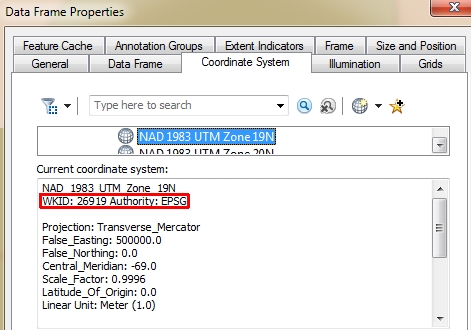
Figure G.1: An ArcGIS dataframe coordinate system properties window. Note the WKID/EPSG code of 26919 (highlighted in red) associated with the NAD 1983 UTM Zone 19 N CS.

That number can then be entered in the http://spatialreference.org/ref/’s search box to pull the Proj4 parameters (note that you must select Proj4 from the list of syntax options).

Figure G.2: Example of a search result for EPSG 26919 at http://spatialreference.org/ref/. Note that after clicking the EPSG:269191 link, you must then select the Proj4 syntax from a list of available syntaxes to view the projection parameters

Here are examples of a few common projections:

Projection	WKID	Authority	Syntax
UTM NAD 83 Zone 19N	26919	EPSG	+proj=utm +zone=19 +ellps=GRS80 +datum=NAD83 +units=m +no_defs
USA Contiguous albers equal area	102003	ESRI	+proj=aea +lat_1=29.5 +lat_2=45.5 +lat_0=37.5 +lon_0=-96 +x_0=0 +y_0=0 +ellps=GRS80 +datum=NAD83 +units=m +no_defs
Alaska albers equal area	3338	EPSG	+proj=aea +lat_1=55 +lat_2=65 +lat_0=50 +lon_0=-154 +x_0=0 +y_0=0 +ellps=GRS80 +datum=NAD83 +units=m +no_defs
World Robinson	54030	ESRI	+proj=robin +lon_0=0 +x_0=0 +y_0=0 +ellps=WGS84 +datum=WGS84 +units=m +no_defs

Transforming coordinate systems

The last section showed you how to define or modify the coordinate system definition. This section shows you how to transform the coordinate values associated with the spatial object to a different coordinate system. This process calculates new coordinate values for the points or vertices defining the spatial object.

For example, to transform the s.sf vector object to a WGS 1984 geographic (long/lat) coordinate system, we’ll use the st_transform function.

s.sf.gcs <- st_transform(s.sf, "+proj=longlat +datum=WGS84")
st_crs(s.sf.gcs)

Coordinate Reference System:
  User input: +proj=longlat +datum=WGS84 
  wkt:
GEOGCRS["unknown",
    DATUM["World Geodetic System 1984",
        ELLIPSOID["WGS 84",6378137,298.257223563,
            LENGTHUNIT["metre",1]],
        ID["EPSG",6326]],
    PRIMEM["Greenwich",0,
        ANGLEUNIT["degree",0.0174532925199433],
        ID["EPSG",8901]],
    CS[ellipsoidal,2],
        AXIS["longitude",east,
            ORDER[1],
            ANGLEUNIT["degree",0.0174532925199433,
                ID["EPSG",9122]]],
        AXIS["latitude",north,
            ORDER[2],
            ANGLEUNIT["degree",0.0174532925199433,
                ID["EPSG",9122]]]]

Using the EPSG code equivalent (4326) instead of the proj4 string yields:

s.sf.gcs <- st_transform(s.sf, 4326)
st_crs(s.sf.gcs)

Coordinate Reference System:
  User input: EPSG:4326 
  wkt:
GEOGCRS["WGS 84",
    ENSEMBLE["World Geodetic System 1984 ensemble",
        MEMBER["World Geodetic System 1984 (Transit)"],
        MEMBER["World Geodetic System 1984 (G730)"],
        MEMBER["World Geodetic System 1984 (G873)"],
        MEMBER["World Geodetic System 1984 (G1150)"],
        MEMBER["World Geodetic System 1984 (G1674)"],
        MEMBER["World Geodetic System 1984 (G1762)"],
        MEMBER["World Geodetic System 1984 (G2139)"],
        ELLIPSOID["WGS 84",6378137,298.257223563,
            LENGTHUNIT["metre",1]],
        ENSEMBLEACCURACY[2.0]],
    PRIMEM["Greenwich",0,
        ANGLEUNIT["degree",0.0174532925199433]],
    CS[ellipsoidal,2],
        AXIS["geodetic latitude (Lat)",north,
            ORDER[1],
            ANGLEUNIT["degree",0.0174532925199433]],
        AXIS["geodetic longitude (Lon)",east,
            ORDER[2],
            ANGLEUNIT["degree",0.0174532925199433]],
    USAGE[
        SCOPE["Horizontal component of 3D system."],
        AREA["World."],
        BBOX[-90,-180,90,180]],
    ID["EPSG",4326]]

This approach may add a few more tags (These reflect changes in datum definitions in newer versions of the PROJ library) but, the coordinate values should be the same

To transform a raster object, use the project() function.

elev.r.gcs <- project(elev.r, y="+proj=longlat +datum=WGS84")
st_crs(elev.r.gcs)

Coordinate Reference System:
  User input: GEOGCRS["unknown",
    DATUM["World Geodetic System 1984",
        ELLIPSOID["WGS 84",6378137,298.257223563,
            LENGTHUNIT["metre",1]],
        ID["EPSG",6326]],
    PRIMEM["Greenwich",0,
        ANGLEUNIT["degree",0.0174532925199433],
        ID["EPSG",8901]],
    CS[ellipsoidal,2],
        AXIS["longitude",east,
            ORDER[1],
            ANGLEUNIT["degree",0.0174532925199433,
                ID["EPSG",9122]]],
        AXIS["latitude",north,
            ORDER[2],
            ANGLEUNIT["degree",0.0174532925199433,
                ID["EPSG",9122]]]] 
  wkt:
GEOGCRS["unknown",
    DATUM["World Geodetic System 1984",
        ELLIPSOID["WGS 84",6378137,298.257223563,
            LENGTHUNIT["metre",1]],
        ID["EPSG",6326]],
    PRIMEM["Greenwich",0,
        ANGLEUNIT["degree",0.0174532925199433],
        ID["EPSG",8901]],
    CS[ellipsoidal,2],
        AXIS["longitude",east,
            ORDER[1],
            ANGLEUNIT["degree",0.0174532925199433,
                ID["EPSG",9122]]],
        AXIS["latitude",north,
            ORDER[2],
            ANGLEUNIT["degree",0.0174532925199433,
                ID["EPSG",9122]]]]

If an EPSG code is to be used, adopt the "+init=EPSG: ..." syntax used earlier in this tutorial.

elev.r.gcs <- project(elev.r, y="+init=EPSG:4326")
st_crs(elev.r.gcs)

Coordinate Reference System:
  User input: WGS 84 
  wkt:
GEOGCRS["WGS 84",
    ENSEMBLE["World Geodetic System 1984 ensemble",
        MEMBER["World Geodetic System 1984 (Transit)",
            ID["EPSG",1166]],
        MEMBER["World Geodetic System 1984 (G730)",
            ID["EPSG",1152]],
        MEMBER["World Geodetic System 1984 (G873)",
            ID["EPSG",1153]],
        MEMBER["World Geodetic System 1984 (G1150)",
            ID["EPSG",1154]],
        MEMBER["World Geodetic System 1984 (G1674)",
            ID["EPSG",1155]],
        MEMBER["World Geodetic System 1984 (G1762)",
            ID["EPSG",1156]],
        MEMBER["World Geodetic System 1984 (G2139)",
            ID["EPSG",1309]],
        ELLIPSOID["WGS 84",6378137,298.257223563,
            LENGTHUNIT["metre",1],
            ID["EPSG",7030]],
        ENSEMBLEACCURACY[2.0],
        ID["EPSG",6326]],
    PRIMEM["Greenwich",0,
        ANGLEUNIT["degree",0.0174532925199433],
        ID["EPSG",8901]],
    CS[ellipsoidal,2],
        AXIS["longitude",east,
            ORDER[1],
            ANGLEUNIT["degree",0.0174532925199433,
                ID["EPSG",9122]]],
        AXIS["latitude",north,
            ORDER[2],
            ANGLEUNIT["degree",0.0174532925199433,
                ID["EPSG",9122]]],
    USAGE[
        SCOPE["unknown"],
        AREA["World."],
        BBOX[-90,-180,90,180]]]

A geographic coordinate system is often desired when overlapping a layer with a web based mapping service such as Google, Bing or OpenStreetMap (even though these web based services end up projecting to a projected coordinate system–most likely a Web Mercator projection). To check that s.sf.gcs was properly transformed, we’ll overlay it on top of an OpenStreetMap using the leaflet package.

library(leaflet)
leaflet(s.sf.gcs) %>% 
  addPolygons() %>% 
  addTiles()

Next, we’ll explore other transformations using a tmap dataset of the world

library(tmap)
data(World)  # The dataset is stored as an sf object
 
# Let's check its current coordinate system
st_crs(World)

Coordinate Reference System:
  User input: EPSG:4326 
  wkt:
GEOGCRS["WGS 84",
    DATUM["World Geodetic System 1984",
        ELLIPSOID["WGS 84",6378137,298.257223563,
            LENGTHUNIT["metre",1]]],
    PRIMEM["Greenwich",0,
        ANGLEUNIT["degree",0.0174532925199433]],
    CS[ellipsoidal,2],
        AXIS["geodetic latitude (Lat)",north,
            ORDER[1],
            ANGLEUNIT["degree",0.0174532925199433]],
        AXIS["geodetic longitude (Lon)",east,
            ORDER[2],
            ANGLEUNIT["degree",0.0174532925199433]],
    USAGE[
        SCOPE["unknown"],
        AREA["World"],
        BBOX[-90,-180,90,180]],
    ID["EPSG",4326]]

The following chunk transforms the world map to a custom azimuthal equidistant projection centered on latitude 0 and longitude 0. Here, we’ll use the proj4 syntax.

World.ae <- st_transform(World, "+proj=aeqd +lat_0=0 +lon_0=0 +x_0=0 +y_0=0 +ellps=WGS84 +datum=WGS84 +units=m +no_defs")

Let’s check the CRS of the newly created vector layer

st_crs(World.ae) 

Coordinate Reference System:
  User input: +proj=aeqd +lat_0=0 +lon_0=0 +x_0=0 +y_0=0 +ellps=WGS84 +datum=WGS84 +units=m +no_defs 
  wkt:
PROJCRS["unknown",
    BASEGEOGCRS["unknown",
        DATUM["World Geodetic System 1984",
            ELLIPSOID["WGS 84",6378137,298.257223563,
                LENGTHUNIT["metre",1]],
            ID["EPSG",6326]],
        PRIMEM["Greenwich",0,
            ANGLEUNIT["degree",0.0174532925199433],
            ID["EPSG",8901]]],
    CONVERSION["unknown",
        METHOD["Modified Azimuthal Equidistant",
            ID["EPSG",9832]],
        PARAMETER["Latitude of natural origin",0,
            ANGLEUNIT["degree",0.0174532925199433],
            ID["EPSG",8801]],
        PARAMETER["Longitude of natural origin",0,
            ANGLEUNIT["degree",0.0174532925199433],
            ID["EPSG",8802]],
        PARAMETER["False easting",0,
            LENGTHUNIT["metre",1],
            ID["EPSG",8806]],
        PARAMETER["False northing",0,
            LENGTHUNIT["metre",1],
            ID["EPSG",8807]]],
    CS[Cartesian,2],
        AXIS["(E)",east,
            ORDER[1],
            LENGTHUNIT["metre",1,
                ID["EPSG",9001]]],
        AXIS["(N)",north,
            ORDER[2],
            LENGTHUNIT["metre",1,
                ID["EPSG",9001]]]]

Here’s the mapped output:

tm_shape(World.ae) + tm_fill() 

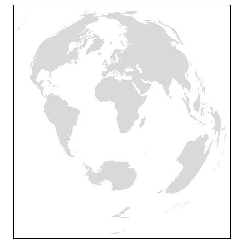
The following chunk transforms the world map to an Azimuthal equidistant projection centered on Maine, USA (69.8° West, 44.5° North) .

World.aemaine <- st_transform(World, "+proj=aeqd +lat_0=44.5 +lon_0=-69.8 +x_0=0 +y_0=0 +ellps=WGS84 +datum=WGS84 +units=m +no_defs")

tm_shape(World.aemaine) + tm_fill()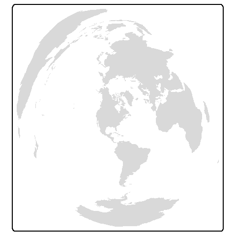  

The following chunk transforms the world map to a World Robinson projection.

World.robin <- st_transform(World,"+proj=robin +lon_0=0 +x_0=0 +y_0=0 +ellps=WGS84 +datum=WGS84 +units=m +no_defs")
tm_shape(World.robin) + tm_fill()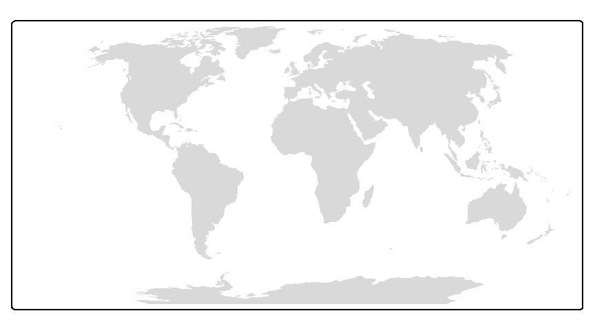  

The following chunk transforms the world map to a World sinusoidal projection.

World.sin <- st_transform(World,"+proj=sinu +lon_0=0 +x_0=0 +y_0=0 +ellps=WGS84 +datum=WGS84 +units=m +no_defs")
tm_shape(World.sin) + tm_fill()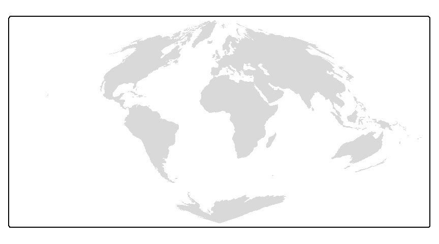  

The following chunk transforms the world map to a World Mercator projection.

World.mercator <- st_transform(World,"+proj=merc +lon_0=0 +k=1 +x_0=0 +y_0=0 +ellps=WGS84 +datum=WGS84 +units=m +no_defs")
tm_shape(World.mercator) + tm_fill()  

Reprojecting to a new meridian center

An issue that can come up when transforming spatial data is when the location of the tangent line(s) or points in the CS definition forces polygon features to be split across the 180° meridian. For example, re-centering the Mercator projection to -69° will create the following output.

World.mercator2 <- st_transform(World, "+proj=merc +lon_0=-69 +k=1 +x_0=0 +y_0=0 +ellps=WGS84 +datum=WGS84 +units=m +no_defs")

tm_shape(World.mercator2) + tm_borders()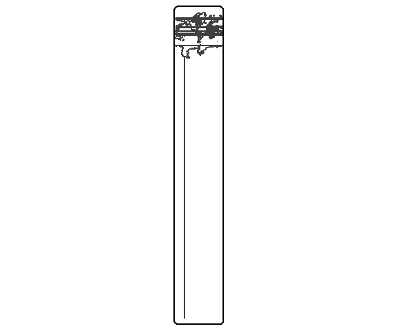

The polygons are split and R does not know how to piece them together.

One solution is to split the polygons at the new meridian using the st_break_antimeridian function before projecting to a new re-centered coordinate system.

# Define new meridian
meridian2 <- -69

# Split world at new meridian
wld.new <- st_break_antimeridian(World, lon_0 = meridian2)

# Now reproject to Mercator using new meridian center
wld.merc2 <- st_transform(wld.new, 
                          paste("+proj=merc +lon_0=", meridian2 ,
                                "+k=1 +x_0=0 +y_0=0 +ellps=WGS84 +datum=WGS84 +units=m +no_defs") )

tm_shape(wld.merc2) + tm_borders()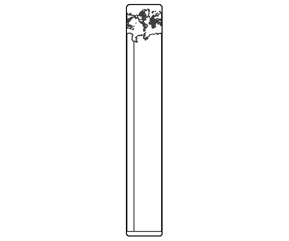

This technique can be applied to any other projections. Here’s an example of a Robinson projection.

wld.rob.sf <-  st_transform(wld.new, 
                            paste("+proj=robin +lon_0=", meridian2 ,
                                  "+k=1 +x_0=0 +y_0=0 +ellps=WGS84 +datum=WGS84 +units=m +no_defs") )
tm_shape(wld.rob.sf) + tm_borders()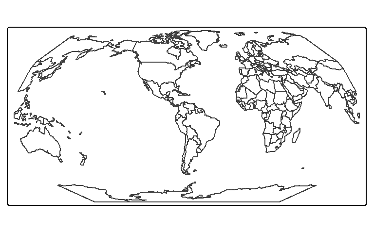

A note about containment

While in theory, a point completely enclosed by a bounded area should always remain bounded by that area in any projection, this is not always the case in practice. This is because the transformation applies to the vertices that define the line segments and not the lines themselves. So if a point is inside of a polygon and very close to one of its boundaries in its native projection, it may find itself on the other side of that line segment in another projection hence outside of that polygon. In the following example, a polygon layer and point layer are created in a Miller coordinate system where the points are enclosed in the polygons.

# Define a few projections
miller <- "+proj=mill +lat_0=0 +lon_0=0 +x_0=0 +y_0=0 +ellps=WGS84 +datum=WGS84 +units=m +no_defs"
lambert <- "+proj=lcc +lat_1=20 +lat_2=60 +lat_0=40 +lon_0=-96 +x_0=0 +y_0=0 +ellps=GRS80 +datum=NAD83 +units=m +no_defs"

# Subset the World data layer and reproject to Miller
wld.mil <- subset(World, iso_a3 == "CAN" | iso_a3 == "USA") |>
  st_transform(miller)

# Create polygon and point layers in the Miller projection  
sf1 <- st_sfc( st_polygon(list(cbind(c(-13340256,-13340256,-6661069, -6661069, -13340256),
                               c(7713751, 5326023, 5326023,7713751, 7713751 )))), crs = miller) 

pt1 <- st_sfc( st_multipoint(rbind(c(-11688500,7633570), c(-11688500,5375780),
                                  c(-10018800,7633570), c(-10018800,5375780),
                                  c(-8348960,7633570), c(-8348960,5375780))),  crs = miller)
pt1 <- st_cast(pt1, "POINT") # Create single part points

# Plot the data layers in their native projection
tm_shape(wld.mil) +tm_fill(col="grey") + 
  tm_graticules(x = c(-60,-80,-100, -120, -140), 
                y = c(30,45, 60), 
                labels.col = "white", col="grey90") +
  tm_shape(sf1) + tm_polygons("red", alpha = 0.5, border.col = "yellow") +
  tm_shape(pt1) + tm_dots(size=0.2)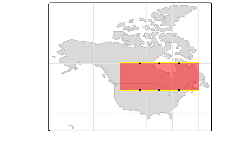 

The points are close to the boundaries, but they are inside of the polygon nonetheless. To confirm, we can run st_contains on the dataset:

st_contains(sf1, pt1)

Sparse geometry binary predicate list of length 1,
where the predicate was `contains'
 1: 1, 2, 3, 4, 5, 6

All six points are selected, as expected.

Now, let’s reproject the data into a Lambert conformal projection.

# Transform the data
wld.lam <- st_transform(wld.mil, lambert)
pt1.lam <- st_transform(pt1, lambert)
sf1.lam <- st_transform(sf1, lambert)

# Plot the data in the Lambert coordinate system
tm_shape(wld.lam) +tm_fill(col="grey") + 
  tm_graticules( x = c(-60,-80,-100, -120, -140), 
                 y = c(30,45, 60), 
                 labels.col = "white", col="grey90") +
  tm_shape(sf1.lam) + tm_polygons("red", alpha = 0.5, border.col = "yellow") +
  tm_shape(pt1.lam) + tm_dots(size=0.2)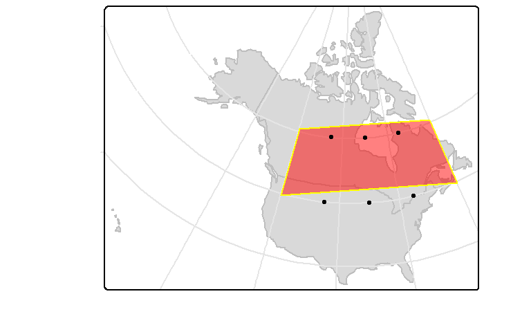   

Only three of the points are contained. We can confirm this using the st_contains function:

st_contains(sf1.lam, pt1.lam)

Sparse geometry binary predicate list of length 1,
where the predicate was `contains'
 1: 1, 3, 5

To resolve this problem, one should densify the polygon by adding more vertices along the line segment. The vertices density will be dictated by the resolution needed to preserve the map’s containment properties and is best determined experimentally.

We’ll use the st_segmentize function to create vertices at 1 km (1000 m) intervals.

# Add vertices every 1000 meters along the polygon's line segments
sf2 <- st_segmentize(sf1, 1000)

# Transform the newly densified polygon layer
sf2.lam <- st_transform(sf2, lambert)

# Plot the data
tm_shape(wld.lam) + tm_fill(col="grey") + 
  tm_graticules( x = c(-60,-80,-100, -120, -140), 
                 y = c(30,45, 60), 
                 labels.col = "white", col="grey90") +
  tm_shape(sf2.lam) + tm_polygons("red", alpha = 0.5, border.col = "yellow") +
  tm_shape(pt1.lam) + tm_dots(size=0.2)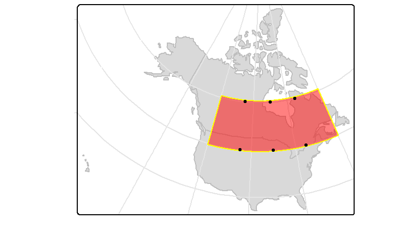 

Now all points remain contained by the polygon. We can check via:

st_contains(sf2.lam, pt1.lam)

Sparse geometry binary predicate list of length 1,
where the predicate was `contains'
 1: 1, 2, 3, 4, 5, 6

Creating Tissot indicatrix circles

Most projections will distort some aspect of a spatial property, especially area and shape. A nice way to visualize the distortion afforded by a projection is to create geodesic circles.

First, create a point layer that will define the circle centers in a lat/long coordinate system.

tissot.pt <- st_sfc( st_multipoint(rbind(c(-60,30), c(-60,45), c(-60,60),
                                  c(-80,30), c(-80,45), c(-80,60),
                                  c(-100,30), c(-100,45), c(-100,60),
                                  c(-120,30), c(-120,45), c(-120,60) )),  crs = "+proj=longlat")
tissot.pt <- st_cast(tissot.pt, "POINT") # Create single part points

Next we’ll construct geodesic circles from these points using the geosphere package.

library(geosphere)

cr.pt <- list() # Create an empty list

# Loop through each point in tissot.pt and generate 360 vertices at 300 km
# from each point in all directions at 1 degree increment. These vertices
# will be used to approximate the Tissot circles
for (i in 1:length(tissot.pt)){
  cr.pt[[i]] <- list( destPoint( as(tissot.pt[i], "Spatial"), b=seq(0,360,1), d=300000) )
}

# Create a closed polygon from the previously generated vertices
tissot.sfc <- st_cast( st_sfc(st_multipolygon(cr.pt ),crs = "+proj=longlat"), "POLYGON" )

We’ll check that these are indeed geodesic circles by computing the geodesic area of each polygon. We’ll use the st_area function from sf which will revert to geodesic area calculation if a lat/long coordinate system is present.

tissot.sf <- st_sf( geoArea =  st_area(tissot.sfc), tissot.sfc )

The true area of the circles should be \(\pi * r^2\) or 2.8274334^{11} square meters in our example. Let’s compute the error in the tissot output. The values will be reported as fractions.

( (pi * 300000^2) -  as.vector(tissot.sf$geoArea) ) / (pi * 300000^2)

 [1] -0.0008937164  0.0024530577  0.0057943110 -0.0008937164
 [5]  0.0024530577  0.0057943110 -0.0008937164  0.0024530577
 [9]  0.0057943110 -0.0008937164  0.0024530577  0.0057943110

In all cases, the error is less than 0.1%. The error is primarily due to the discretization of the circle parameter.

Let’s now take a look at the distortions associated with a few popular coordinate systems. We’ll start by exploring the Mercator projection.

# Transform geodesic circles and compute area error as a percentage
tissot.merc <- st_transform(tissot.sf, "+proj=merc +ellps=WGS84")
tissot.merc$area_err <- round((st_area(tissot.merc, tissot.merc$geoArea)) / 
                                tissot.merc$geoArea * 100 , 2)

# Plot the map
tm_shape(World, bbox = st_bbox(tissot.merc), projection = st_crs(tissot.merc)) + 
  tm_borders() + 
  tm_shape(tissot.merc) + tm_polygons(col="grey", border.col = "red", alpha = 0.3) + 
  tm_graticules(x = c(-60,-80,-100, -120, -140), 
                y = c(30,45, 60),
               labels.col = "white", col="grey80") +
  tm_text("area_err", size=.8, alpha=0.8, col="blue")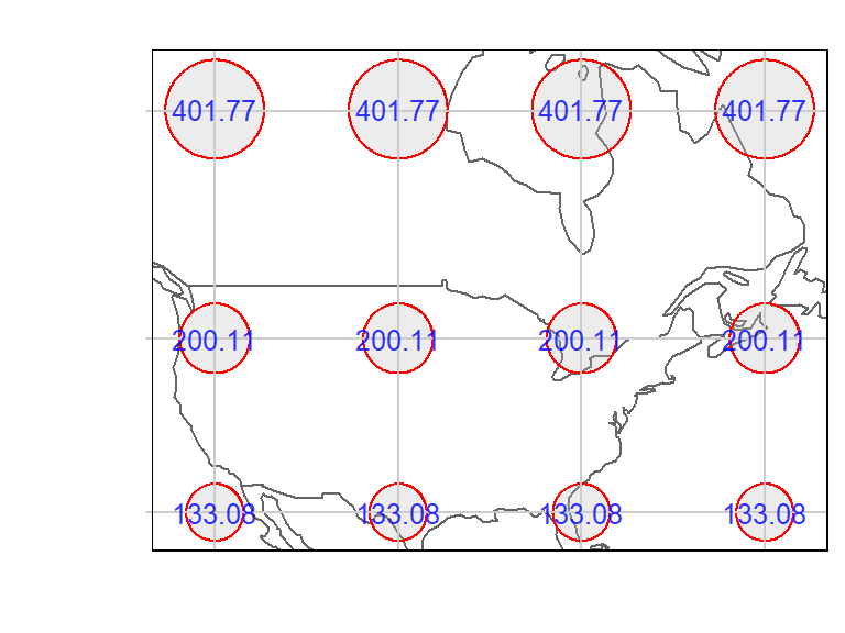

The mercator projection does a good job at preserving shape, but the area’s distortion increases dramatically poleward.

Next, we’ll explore the Lambert azimuthal equal area projection centered at 45 degrees north and 100 degrees west.

# Transform geodesic circles and compute area error as a percentage
tissot.laea <- st_transform(tissot.sf, "+proj=laea +lat_0=45 +lon_0=-100 +ellps=WGS84")
tissot.laea$area_err <- round( (st_area(tissot.laea ) - tissot.laea$geoArea) / 
                                 tissot.laea$geoArea * 100, 2)

# Plot the map
tm_shape(World, bbox = st_bbox(tissot.laea), projection = st_crs(tissot.laea)) + 
  tm_borders() + 
  tm_shape(tissot.laea) + tm_polygons(col="grey", border.col = "red", alpha = 0.3) + 
  tm_graticules(x=c(-60,-80,-100, -120, -140), 
           y = c(30,45, 60),
           labels.col = "white", col="grey80") +
  tm_text("area_err", size=.8, alpha=0.8, col="blue")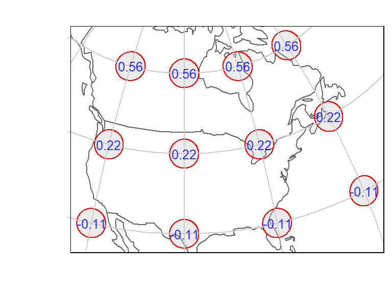

The area error across the 48 states is near 0. But note that the shape does become slightly distorted as we move away from the center of projection.

Next, we’ll explore the Robinson projection.

# Transform geodesic circles and compute area error as a percentage
tissot.robin <- st_transform(tissot.sf, "+proj=robin  +ellps=WGS84")
tissot.robin$area_err <- round(  (st_area(tissot.robin ) - tissot.robin$geoArea) / 
                                   tissot.robin$geoArea * 100, 2)

# Plot the map
tm_shape(World, bbox = st_bbox(tissot.robin), projection = st_crs(tissot.robin)) + 
  tm_borders() + 
  tm_shape(tissot.robin) + tm_polygons(col="grey", border.col = "red", alpha = 0.3) + 
  tm_graticules(x=c(-60,-80,-100, -120, -140), 
                y = c(30,45, 60),
                labels.col = "white", col="grey80") +
  tm_text("area_err", size=.8, alpha=0.8, col="blue")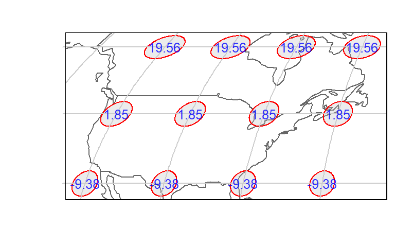

Both shape and area are measurably distorted for the north american continent.