Chapter 14 First-Order Point Pattern Analysis: Modeling Spatial Intensity

14.1 Introduction

In spatial point pattern analysis, first-order effects refer to variations in the intensity of points across a study area due to external factors. These effects describe how the likelihood of observing a point changes from one location to another, independent of the presence or absence of other points. For example, oak trees may be more densely distributed in areas with favorable soil conditions, or retail stores may cluster in regions with higher population density. In both cases, the spatial variation is driven by underlying environmental or socioeconomic covariates rather than interactions between the points themselves.

This chapter focuses on techniques for detecting and modeling these first-order effects. We begin with simple descriptive tools such as global and local density measures, then move to more refined methods like kernel density estimation and covariate-adjusted intensity modeling. Finally, we introduce statistical models, such as the Poisson point process, that allow us to formally test hypotheses about how external variables influence point intensity. By isolating first-order effects, we lay the groundwork for more advanced analyses of second-order properties, which examine how points interact with one another.

14.2 Centrography

Before diving into formal models of spatial intensity, it’s helpful to begin with simple descriptive tools that summarize the overall distribution of points. This approach, known as centrography, includes techniques such as the mean center, standard distance and standard deviational ellipse. These measures provide insight into the central tendency and dispersion of a point pattern, offering a useful starting point for exploring spatial variation.

These point pattern analysis techniques were popular before computers were ubiquitous as hand calculations were relatively simple. However, these summary statistics are too concise and hide far more valuable information about the observed pattern.

In the following sections, we introduce density-based methods as a bridge between raw spatial data and more formal modeling of intensity.

14.3 Understanding Intensity and Density in Point Patterns

In point pattern analysis, the terms intensity and density are closely related but conceptually distinct. Understanding the difference is important when interpreting spatial patterns and building models.

• Density refers to the observed number of points per unit area in a dataset. It’s a descriptive statistic–what we actually count from the data. For example, if there are 31 trees in a 100 square meter plot, the density is 0.31 trees per square meter.

• Intensity, on the other hand, refers to the underlying rate or likelihood that a point occurs at a location. It’s a property of the process that generated the pattern, not just the pattern itself. Intensity is often denoted by the symbol \(\lambda\) and can vary across space. When we estimate intensity from observed data, we use \(\widehat{\lambda}\) to indicate that it’s an approximation.

Think of it this way: density is what we observe, intensity is what we infer. If the intensity is constant across the study area, we say the process is homogeneous, if it varies, the process is inhomogeneous. We therefore need tools that can model how intensity changes with location or covariates.

14.4 Global density

A basic estimate of a point pattern’s intensity, \(\widehat{\lambda}\), is its global density–the average number of points per unit area across the entire study region. It is computed as the ratio of the total number of observed points, \(n\), to the surface area of the study region, \(a\):

\(\begin{equation} \widehat{\lambda} = \frac{n}{a} \label{eq:global-density} \end{equation}\)

This estimate assumes that the underlying process is homogeneous, meaning the intensity is constant throughout the region.

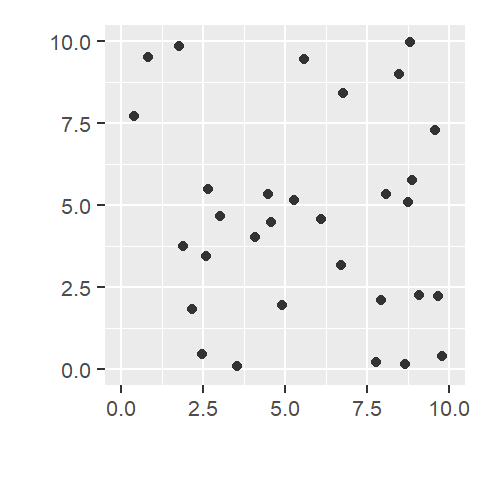
Figure 14.1: An example of a point pattern where n = 31 and the study area (defined by a square boundary) is 10 units squared. The point density is thus 31/100 = 0.31 points per unit area.

While useful as a summary statistic, global density can mask important spatial variation, which motivates the need for local density measures introduced in the next section.

14.5 Local density

A point pattern’s density can vary across space, and measuring it at different locations allows us to assess whether the underlying process’s local intensity, \(\widehat{\lambda}_i\), is spatially uniform or not. This spatial variation is a key aspect of first-order effects, where external factors may influence the likelihood of observing a point in different parts of the study area.

Identifying non-uniform intensity is important because it can confound distance-based analyses (covered in the next chapter) which assume stationarity–the assumption that the underlying process generating the points has a constant intensity across the study area.

Several techniques are available for estimating local density. In this chapter, we focus on two widely used methods: quadrat density, which divides the study area into discrete subregions, and kernel density, which uses a moving window to produce a smooth surface of estimated intensity.

14.5.1 Quadrat density

Quadrat density analysis involves dividing the study area into sub-regions called quadrats. For each quadrat, the local density is computed by dividing the number of points within the quadrat by its area. This provides a spatially localized estimate of point intensity.

This method assumes that the intensity of the point process is roughly constant within each quadrat, which may not hold if quadrats are too large or poorly aligned with underlying spatial variation.

Quadrats can take various shapes such as hexagons and triangles. In the following example density is computed for square shaped quadrats.

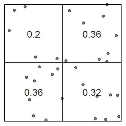
Figure 14.2: An example of a quadrat count where the study area is divided into four equally sized quadrats whose area is 25 square units each. The density in each quadrat can be computed by dividing the number of points in each quadrat by that quadrat’s area.

The choice of quadrat numbers and quadrat shape can influence the measure of local density and must be chosen with care. If very small quadrat sizes are used, you risk having many empty quadrats which may prove uninformative. If very large quadrat sizes are used, you risk missing subtle changes in spatial density distributions such as an east-west gradient in density values.

Instead of dividing the study area into uniform shapes, quadrats can also be defined based on an underlying covariate–a spatial variable believed to influence point intensity (e.g., elevation, land cover, or population density). For example, if it’s believed that the underlying point pattern process is driven by elevation, quadrats can be defined by sub-regions such as different ranges of elevation values (labeled 1 through 4 on the right-hand plot in the following example). This can result in quadrats with non-uniform shape and area.

Converting a continuous field into discretized areas is sometimes referred to as tessellation. The end product is a tessellated surface.

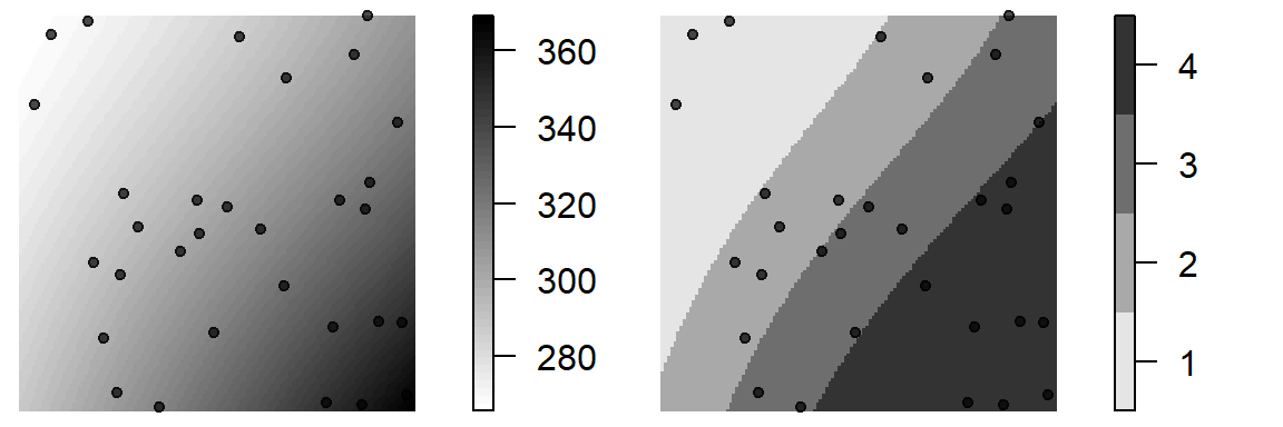
Figure 14.3: Example of a covariate. Figure on the left shows the elevation map. Figure on the right shows elevation broken down into four sub-regions (a tessellated surface) for which local density values will be computed.

If the local intensity changes across the tessellated covariate, then there is evidence of a dependence between the process that generated the point pattern and the covariate. In our example, sub-regions 1 through 4 have surface areas of 23.54, 25.2, 25.21, 26.06 map units respectively. To compute these regions’ point densities, we simply divide the number of points by the respective area values.

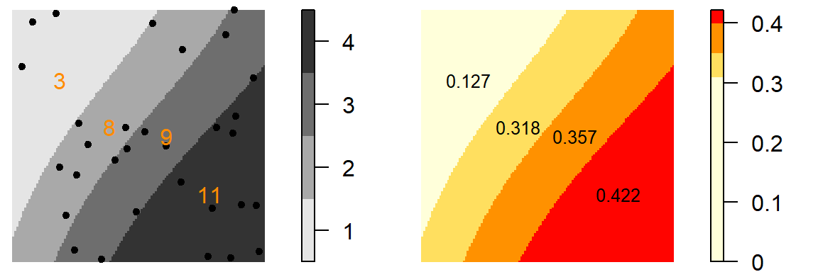
Figure 14.4: Figure on the left displays the number of points in each elevation sub-region (sub-regions are coded as values ranging from 1 to 4). Figure on the right shows the density of points (number of points divided by the area of the sub-region).

We can plot the relationship between point density and elevation regions to help assess any dependence between the variables.

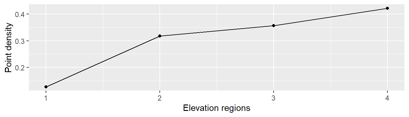
Figure 14.5: Plot of point density vs elevation regions.

It’s important to note that how one chooses to tessellate a surface can have an influence on the resulting density distribution. For example, dividing the elevation into seven sub-regions produces the following density values.

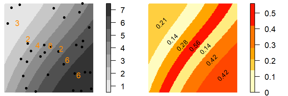
Figure 14.6: Same analysis as last figure using different sub-regions. Note the difference in density distribution.

While the high density in the western part of the study area remains, the density values to the east are no longer consistent across the other three regions.

The quadrat analysis approach has advantages–it is easy to compute and interpret. However, it does suffer from the modifiable areal unit problem (MAUP) as highlighted in the last two examples.

Quadrat density is most useful when the study area can be meaningfully divided into regions of interest, or when a covariate provides a natural way to segment space. However, it may be less effective in detecting subtle or continuous spatial variation, which motivates the use of kernel density methods introduced next.

14.5.2 Kernel density

The kernel density approach is a method for estimating the spatial intensity of a point pattern. Like quadrat density, it computes localized density values, but it does so using a moving window that overlaps across space, producing a smoother and more continuous estimate of intensity.

This moving window is defined by a kernel. A kernel is a mathematical function that defines how much influence each point has on the estimated intensity at a given location.

The kernel density method produces a grid of intensity estimates where each cell’s value reflects the weighted contribution of nearby points within the kernel window centered on that cell.

The simplest kernel function is a basic kernel where each point in the kernel window is assigned equal weight.

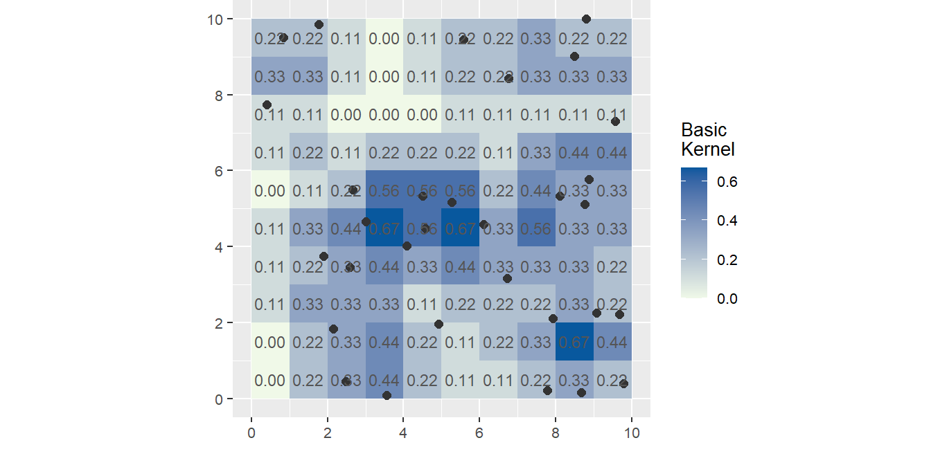
Figure 14.7: An example of a basic 3x3 kernel density map where each point is assigned an equal weight. For example, the cell centered at location x=1.5 and y =7.5 has one point within a 3x3 unit (pixel) region and thus has a local density of 1/9 = 0.11.

More common kernel functions assign weights to points that are inversely proportional to their distances to the kernel window’s center. A few such kernel functions follow a gaussian or quartic like distribution function. These functions tend to produce a smoother density map.

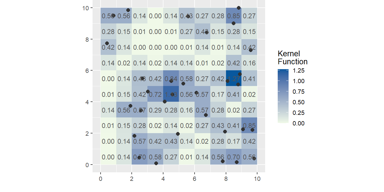
Figure 14.8: An example of a kernel function is the 3x3 quartic kernel function where each point in the kernel window is weighted based on its proximity to the kernel’s center cell (typically, closer points are weighted more heavily). Kernel functions, like the quartic, tend to generate smoother surfaces.

While the basic kernel density approach involves uniformly applying a kernel function across the study area to produce a smooth map of estimated point intensity, its usefulness extends to understanding how this intensity relates to covariates. A common exploratory step is to visually or statistically compare the computed kernel density map with a map of an underlying covariate (such as terrain elevation or population density). This helps identify potential spatial relationships, for instance, observing if areas of high event density tend to correspond with areas of high covariate values.

14.5.3 Non-parametric Intensity Modeling with Covariates

In an earlier section, we learned that we could use a covariate, like elevation, to define the sub-regions (quadrats) within which densities were computed.

Here, instead of dividing the study region into discrete sub-regions, we estimate an intensity function, denoted \(\rho(z)\), that describes how point intensity varies as a function of a covariate \(z\) (e.g., elevation). This function is then used to model the spatial intensity \(\widehat{\lambda}(x)\) at each location \(x\) in the study area.

In this framework, \(\rho(z)\) captures how intensity varies with the covariate, while \(\widehat{\lambda}(x)\) applies this relationship spatially across the study region using the covariate’s spatial distribution.

\(\rho(z)\) can be estimated in one of three different ways–by ratio, re-weight and transform methods. We will not delve into the differences between these methods, but note that there is more than one way to estimate \(\rho(z)\) in the presence of a covariate.

In the following example, the elevation raster is used as the covariate in the \(\rho(z)\) function using the ratio method (The ratio method compares the observed density of points at different covariate values to the density of the covariate itself, producing an estimate of relative intensity). The right-most plot maps the modeled intensity as a function of elevation.

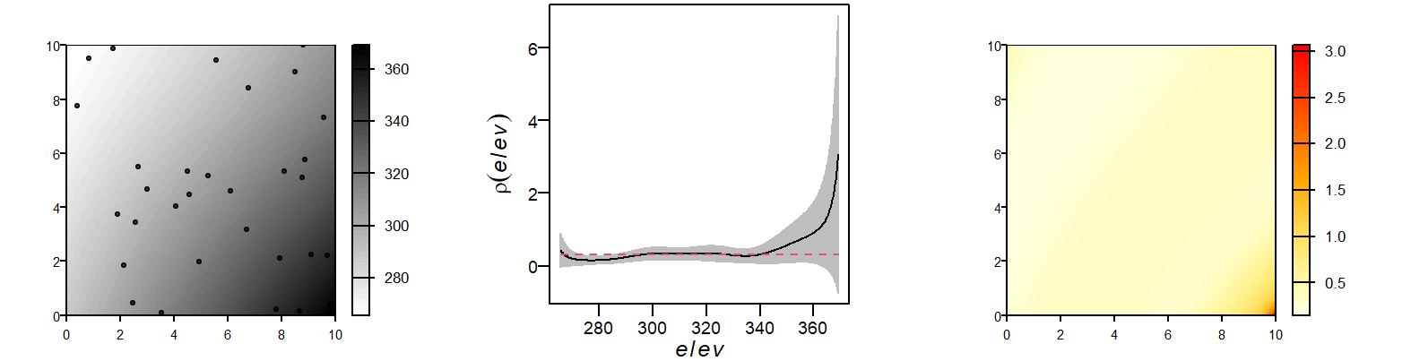
Figure 14.9: An estimate of \(\rho\) using the ratio method. The figure on the left shows the point distribution superimposed on the elevation layer. The middle figure plots the estimated \(\rho\) as a function of elevation. The envelope shows the 95% confidence interval. The figure on the right shows the modeled density of \(\widehat{\lambda}\) which is a function of the elevation raster (i.e. \(\widehat{\lambda}=\widehat{\rho}_{elevation}\)).

We can compare the modeled intensity function to the kernel density function of the observed point pattern via a scatter plot.

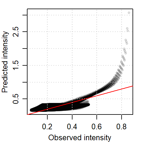
Figure 14.10: Scatter plot of predicted intensity vs. observed kernel density.

A red one-to-one diagonal line is added to the plot. The scatter plot compares the predicted intensity (based on elevation) to the observed kernel density. While the general trend is positive, the relationship is not strictly linear. This deviation may reflect uncertainty in regions with sparse data, such as high elevations, where fewer points lead to less reliable estimates. This uncertainty is very apparent in the \(\rho_{elev}\) vs. elevation plot of 14.9 where the 95% confidence interval envelope widens at higher elevation values (indicating the greater uncertainty in our estimated \(\rho\) value at those higher elevation values). The widening of the confidence envelope at higher elevations reflects increased uncertainty due to fewer observations in those regions–a common issue in spatial modeling when covariate values are unevenly distributed.

Modeling intensity as a function of a covariate allows us to explore first-order effects more rigorously. It helps determine whether external factors–like elevation or population density–can explain the spatial distribution of points.

Note that this method, while still utilizing kernel-based techniques, offers a more integrated approach than the basic kernel density estimation described in the previous section. In that method, we first produce a map of point density (by uniformly applying a kernel over each event) that can then be compared to a covariate map to identify potential associations. Here, however, the process is conceptually different: we use kernel-based methods to directly model how the point intensity varies as a function of a covariate. This means the covariate itself is woven into the estimation, allowing the kernel to effectively adapt its smoothing, or its contribution to the density estimate, so that the resulting intensity map inherently reflects the covariate’s influence.

This approach provides a non-parametric estimate of how point intensity varies with a covariate, offering insight into first-order effects. The function \(\rho(z)\) captures this relationship without assuming a specific parametric form. In the next section, we explore a complementary approach–Poisson point process modeling–which allows us to formally specify intensity as a log-linear function of covariates.

14.5.4 Parametric Intensity Modeling with Covariates

Up to this point, we have focused on techniques that describe the distribution of points across a region of interest. However, it is often more insightful to model the relationship between point locations and an underlying covariate using a formal statistical framework. This can be done by exploring the changes in point density as a function of a covariate, however, unlike techniques explored thus far, this approach makes use of a statistical model. One such model is a Poisson point process model (PPM) which can take the form:

\[ \begin{equation} \lambda(i) = e^{\alpha + \beta Z(i)} \label{eq:density-covariate} \end{equation} \]

This equation defines how the expected number of points per unit area (intensity) varies as a function of the covariate \(Z(i)\). The term \(\lambda(i)\) is the modeled intensity at location \(i\), \(e^{\alpha}\) (the exponent of \(\alpha\)) is the base intensity when the covariate is zero and \(e^{\beta}\) is the multiplier by which the intensity increases (or decreases) for each 1 unit increase in the covariate \(Z(i)\). The parameters \(\alpha\) and \(\beta\) are estimated from the data using maximum likelihood, which finds the values that best explain the observed point pattern given the covariate surface. Note that the units of intensity are derived from the coordinate reference system (e.g., stores per square kilometer), and the interpretation of \(\beta\) depends on the scale and units of the covariate.

The equation is a form of a log-linear model, used in spatial statistics to model intensity. While it resembles logistic regression in structure, the left-hand side represents intensity, not probability. Note that taking the log of both sides of the equation yields the more familiar linear regression model where \(\alpha + \beta Z(i)\) is the linear predictor.

Note: While the Poisson point process model uses a log-linear form to model intensity, logistic regression models the probability of occurrence. These two frameworks are related through the transformation \(\lambda = P / (1 - P)\), which leads to: \[ P(i) = \frac{e^{\alpha + \beta Z(i)}}{1 + e^{\alpha + \beta Z(i)}} \] This relationship is useful when interpreting intensity in terms of probability, especially in presence/absence modeling.

This PPM assumes that events occur independently, and that the intensity varies smoothly with the covariate. It does not account for interactions between points (i.e., second-order effects).

Let’s work with the point distribution of Starbucks cafes in the state of Massachusetts. The point pattern clearly exhibits a non-random distribution. It might be helpful to compare this distribution to some underlying covariate such as the population density distribution.

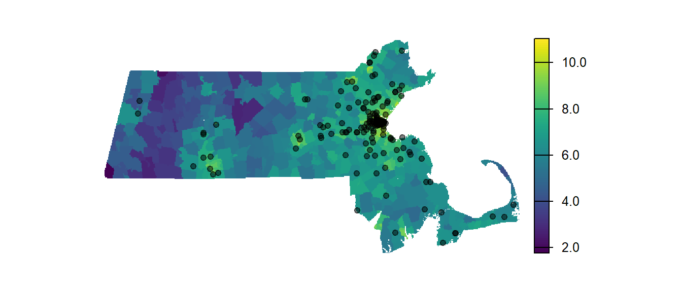
Figure 14.11: Location of Starbucks relative to population density. Note that the classification scheme follows a log scale to more easily differentiate population density values.

We can fit a poisson point process model to these data where the modeled intensity takes on the form:

\[ \begin{equation} Starbucks\ density(i) = e^{\alpha + \beta\ population(i)} \label{eq:walmart-model} \end{equation} \]

The parameters \(\alpha\) and \(\beta\) are estimated from a method called maximum likelihood. Its implementation is not covered here but is widely covered in general statistics text books. The index \((i)\) serves as a reminder that the point density and the population distribution both can vary as a function of location \(i\).

The estimated value for \(\alpha\) in our example is -5.151. This is interpreted as stating that given a population density of zero, the base intensity of the point process is e^-5.151 or 0.00579361 cafes per square kilometer (the units are derived from the point’s reference system)–a number close to zero (as one would expect). The estimated value for \(\beta\) is 0.00017. This is interpreted as stating that for every unit increase in the population density derived from the raster, the intensity of the point process increases by a factor of e^0.00017 or 1.00017.

The plot below shows the fitted intensity curve as a function of population density, along with a confidence envelope. This visualization helps assess whether the relationship is approximately linear and whether uncertainty increases at extreme covariate values.

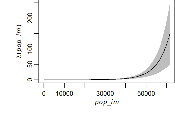
Figure 14.12: Poisson point process model fitted to the relationship between Starbucks store locations and population density. The model assumes a log-linear relationship. Note that the density is reported in number of stores per map unit area (the map units are in kilometers).

In the next section, we explore how to formally compare this covariate-based model to a simpler null model (e.g., homogeneous intensity) using statistical tests. This allows us to assess whether the covariate meaningfully improves our understanding of the spatial distribution of points.

14.6 Hypothesis Testing for Covariate Effects

A Poisson point process model can be fit to any observed point pattern, but fitting a model alone does not guarantee that it provides a meaningful explanation of the spatial distribution. To evaluate whether a covariate-based model improves our understanding of the point pattern, we compare it to a simpler baseline model–typically one that assumes homogeneous intensity across space. In this framework, the homogeneous model serves as the null hypothesis, while the covariate-based model represents the alternative hypothesis.

For example, we may want to assess whether the spatial distribution of Walmart stores is better explained by population density (the alternative hypothesis) than by a model that assumes no spatial preference (the null hypothesis).

Figure 14.13: Location of Walmart stores relative to population density. Note that the classification scheme follows a log scale to more easily differentiate population density values.

To test this, we fit both models to the observed data and compare their performance using a likelihood ratio test.

A Poisson point process model (of the the Walmart point pattern) implemented using spatstat’s ppm function (Baddeley, Rubak, and Turner 2016) produces the following output for the null model:

Stationary Poisson process
Fitted to point pattern dataset 'P'
Intensity: 0.0021276
             Estimate      S.E.   CI95.lo   CI95.hi Ztest     Zval
log(lambda) -6.152761 0.1507557 -6.448236 -5.857285   *** -40.8128

and the following output for the alternative model.

Nonstationary Poisson process
Fitted to point pattern dataset 'P'

Log intensity:  ~pop

Fitted trend coefficients:
  (Intercept)           pop 
-6.2551180493  0.0001043115 

                 Estimate         S.E.       CI95.lo       CI95.hi Ztest
(Intercept) -6.2551180493 1.611991e-01 -6.571062e+00 -5.9391736579   ***
pop          0.0001043115 3.851572e-05  2.882207e-05  0.0001798009    **
                  Zval
(Intercept) -38.803683
pop           2.708284
Problem:
 Values of the covariate 'pop' were NA or undefined at 0.7% (4 out of 572) of 
the quadrature points

Thus, the null model (homogeneous intensity) takes on the form:

\[ \lambda(i) = e^{-6.2} \]

and the alternate model takes on the form:

\[ \lambda(i) = e^{-6.3 + 1.04^{-4}population} \]

To better understand how the two models differ, we can visualize the estimated intensity (\(\widehat{\lambda}\)) as a function of population density for both the null and alternative models.

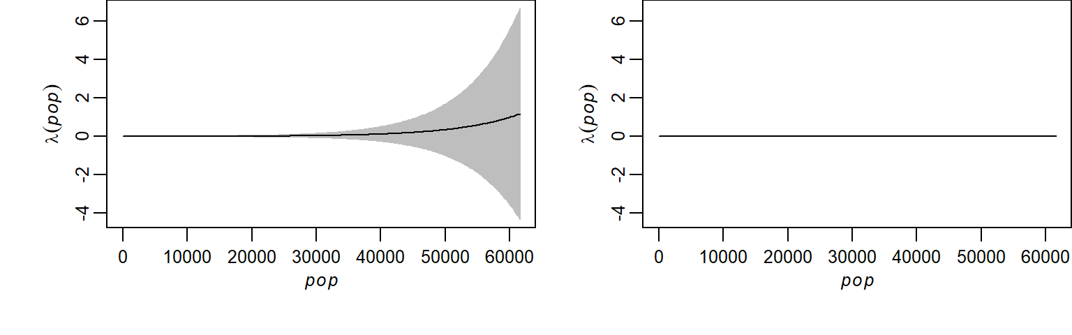
(#fig:f11b_Ho_vs_H)Estimated intensity functions from the Poisson point process model: the left plot shows the covariate-based model (intensity as a function of population density), while the right plot shows the null model (constant intensity). Note the broader confidence interval in the covariate-based model, indicating greater uncertainty at extreme population values (the map units are in kilometers).

The shapes of the fitted model clearly differ between the models, but this does not necessarily imply that the model that includes population density is significantly different from the null model. The relatively wide confidence intervals in the covariate-based model, especially at higher population densities, suggest uncertainty in the estimated relationship. This highlights the importance of formal statistical testing to determine whether the observed differences are meaningful.

To formally assess whether the covariate-based model provides a significantly better fit than the null model, we use a likelihood ratio test. This test compares the log-likelihoods of the two models and evaluates whether the improvement in fit is statistically significant.

Npar	Df	Deviance	Pr(>Chi)
5	NA	NA	NA
6	1	4.253072	0.0391794

The value under the heading PR(>Chi) is the p-value which gives us the probability we would be wrong in rejecting the null. The resulting p-value of 0.039 indicates that, if the null model were true (i.e., if Walmart locations were randomly distributed with constant intensity), there is only a 3.9% chance of observing a pattern that fits the covariate-based model this well. This provides some evidence that population density improves the model’s ability to explain the spatial distribution of Walmart stores.

In summary, the likelihood ratio test suggests that population density is a meaningful covariate in explaining the spatial distribution of Walmart stores, though some uncertainty remains in the estimated relationship.

14.7 Summary

This chapter introduced methods for analyzing first-order properties of spatial point patterns—those driven by external factors rather than interactions between points. We began with descriptive tools such as global and local density measures, including quadrat and kernel density estimation. These methods help identify spatial variation in point intensity and can reveal associations with underlying covariates.

We then explored how covariates can be used to model intensity more formally, both non-parametrically and through parametric approaches like the Poisson point process model (PPM). The PPM allows us to test hypotheses about whether a covariate meaningfully explains the spatial distribution of points, using statistical tools such as the likelihood ratio test.

Importantly, this chapter is limited to first-order effects. While second-order properties—such as point interactions—are central to spatial analysis, they are addressed in the next chapter.

References

Baddeley, Adrian, Ege Rubak, and Rolf Turner. 2016. Spatial Point Patterns, Methodology and Applications with r. Florida: CRC Press.