Residual-Fit Spread Plot — eda

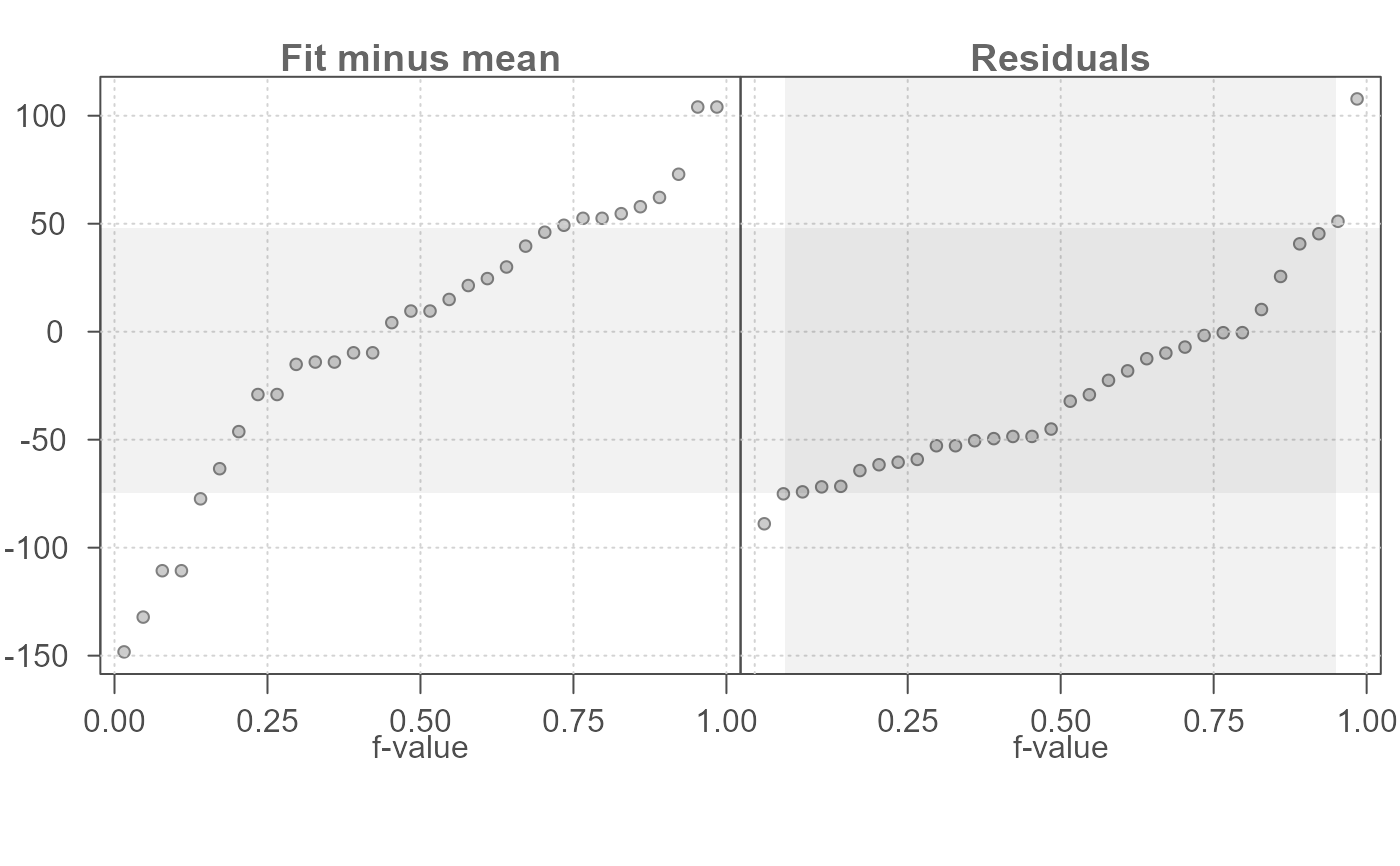
eda_rfs generates a Cleveland residual-fit spread plot for univariate or bivariate data.

Usage

eda_rfs(
  dat,
  x = NULL,
  grp = NULL,
  p = 1L,
  tukey = FALSE,
  show.par = TRUE,
  stat = mean,
  grey = 0.7,
  pch = 21,
  p.col = "grey50",
  p.fill = "grey80",
  inner = 0.9,
  q = FALSE,
  size = 0.8,
  alpha = 0.7,
  ylim = NULL,
  bar = FALSE
)

Arguments

dat: An eda_lm model, an lm model or a dataframe of univariate data.
x: Column of values if dat is a dataframe, ignored otherwise.
grp: Column of categorical variable if dat is a dataframe, ignored otherwise.
p: Power transformation to apply to univariate data. Ignored if linear model is passed to function.
tukey: Boolean determining if a Tukey transformation should be adopted (TRUE) or if a Box-Cox transformation should be adopted (FALSE).
show.par: Boolean determining if the power transformation used with the data should be displayed in the plot's upper-right corner.
stat: Choice of summary statistic to use when centering the fitted values around 0. The stat parameter is also used for fitting univariate values (i.e. for summarizing groups). stat can be either mean or median.
grey: Grey level to apply to plot elements (0 to 1 with 1 = black).
pch: Point symbol type.
p.col: Color for point symbol.
p.fill: Point fill color passed to bg (Only used for pch ranging from 21-25).
inner: Fraction of values that should be captured by the shaded region. Defaults to inner 90% of values.
q: Boolean determining if grey quantile boxes should be plotted.
size: Point size (0-1)
alpha: Point transparency (0 = transparent, 1 = opaque). Only applicable if rgb() is not used to define point colors.
ylim: Define custom y axis limits.
bar: Boolean determining if spread comparison stacked bars should be plotted.

Value

No values are returned

Details

The eda_rfs function generates a residual-fit spread plot for univariate and bivariate data. Input can be a dataframe with one column storing the continuous variable and another column storing the categorical (grouping) variable or, for a bivariate dataset, a model output from an lm(), eda_lm() or eda_rline() function.

The stat argument only applies to univariate data and allows the user to choose the summary statistic to fit to the data (either mean or median). This statistic is also used to recenter the fitted values in the rfs plot.

The q argument, when set to TRUE, will add a shaded region to the residual quantile plot highlighting the mid portion of the data defined by the inner argument (set to 90% of the mid values, by default). The range defined by the mid portion of the data is highlighted in the left plot for comparison with the the full range defined by the fitted values.

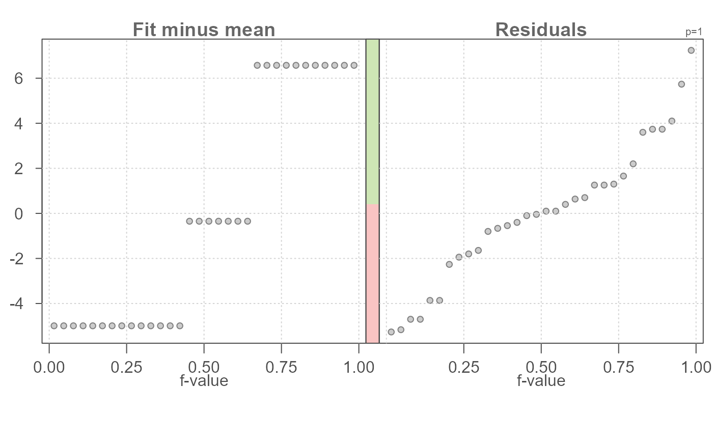
The bar option, when set to TRUE, adds a narrow stacked barplot that compares the spread covered by the residuals (red bar) with the spread covered by the fitted values (green bar). The residual spread is computed for the portion of the residuals defined by the inner argument. The values outputted in the console are those used in computing the vertical bars. The red bar is the relative spread of the residuals and the green bar is the relative spread of the fitted values. The stacked bar plot can be helpful in quickly gauging the effect the fitted values have in explaining the variability in the data. The longer the green bar relative to the red bar, the greater the grouping variable's (for univariate data) or linear model's (for bivariate data) effect in minimizing the uncertainty in the estimated value.

References

William S. Cleveland. Visualizing Data. Hobart Press (1993)
Residual-fit spread article

Examples


# Generate a basic residual-fit spread plot
eda_rfs(mtcars,mpg, cyl)
#> The mid 90.0% of residuals covers about 9.74 units.
#> The fitted values cover a range of 11.56 units, or about 118.7% of the mid 90.0% of residuals.


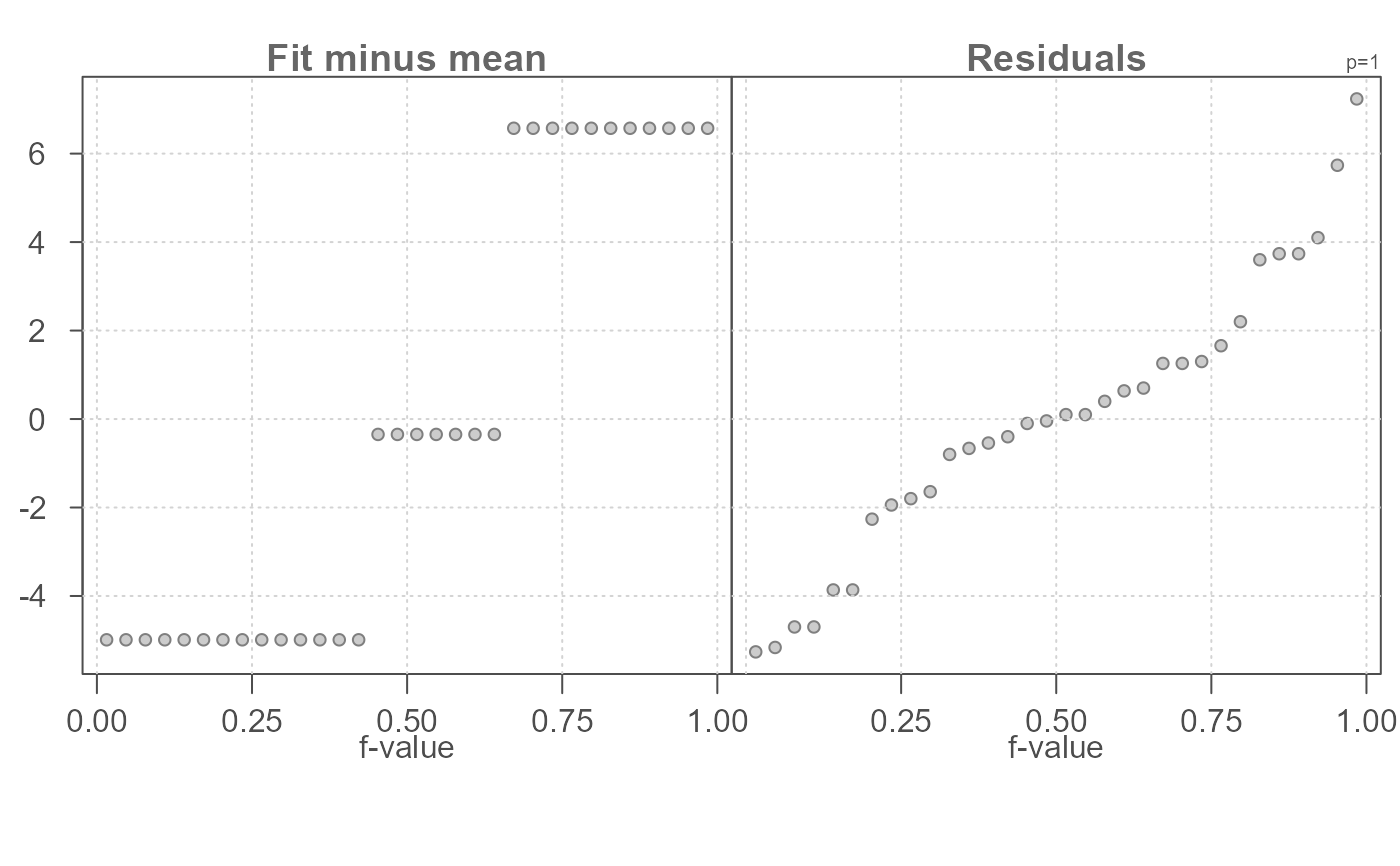# Add inner 90% region to residuals (grey boxes in plot)
# Vertical grey box shows matching y-values
eda_rfs(mtcars,mpg, cyl, q = TRUE)
#> The mid 90.0% of residuals covers about 9.74 units.
#> The fitted values cover a range of 11.56 units, or about 118.7% of the mid 90.0% of residuals.


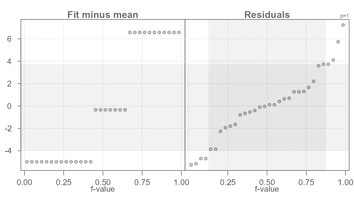
# Change guide to encompass mid 75% of residual values
eda_rfs(mtcars,mpg, cyl, q = TRUE, inner = 0.75)
#> The mid 75.0% of residuals covers about 7.70 units.
#> The fitted values cover a range of 11.56 units, or about 150.1% of the mid 75.0% of residuals.


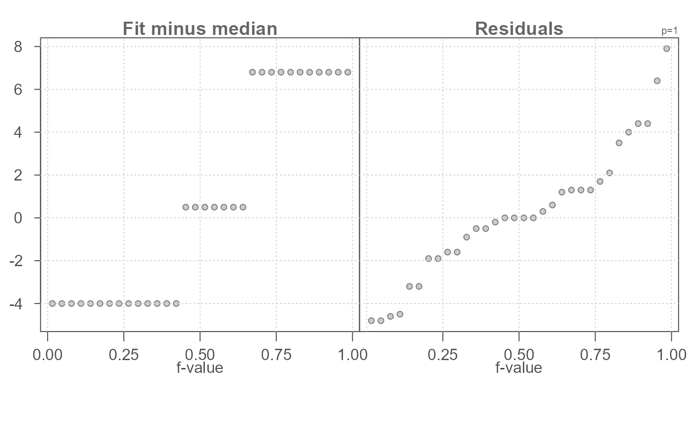
# Use median instead of the mean to compute group summaries and to
# recenter the fitted values around 0.
eda_rfs(mtcars,mpg, cyl, stat = median)
#> The mid 90.0% of residuals covers about 9.99 units.
#> The fitted values cover a range of 10.80 units, or about 108.1% of the mid 90.0% of residuals.


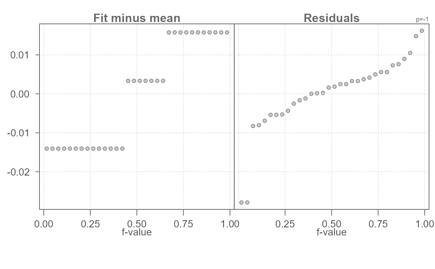
# Apply power transformation of -1 to mpg. Defaults to box-cox method.
eda_rfs(mtcars,mpg, cyl, p = -1)
#> The mid 90.0% of residuals covers about 0.03 units.
#> The fitted values cover a range of 0.03 units, or about 101.0% of the mid 90.0% of residuals.


# Display a stacked bar plot showing relative importance in spreads
# between fitted values and residuals.
eda_rfs(mtcars,mpg, cyl, bar = TRUE)
#> The mid 90.0% of residuals covers about 9.74 units.
#> The fitted values cover a range of 11.56 units, or about 118.7% of the mid 90.0% of residuals.


# Generate rfs plot for bivariate model output. Model can be generated from
# lm(), eda_lm() or eda_rline()
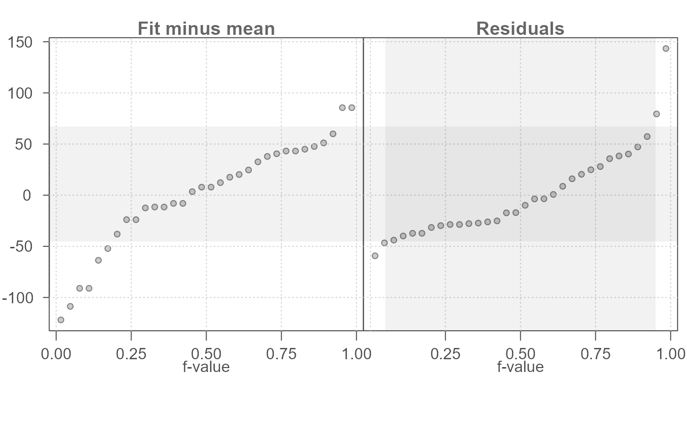
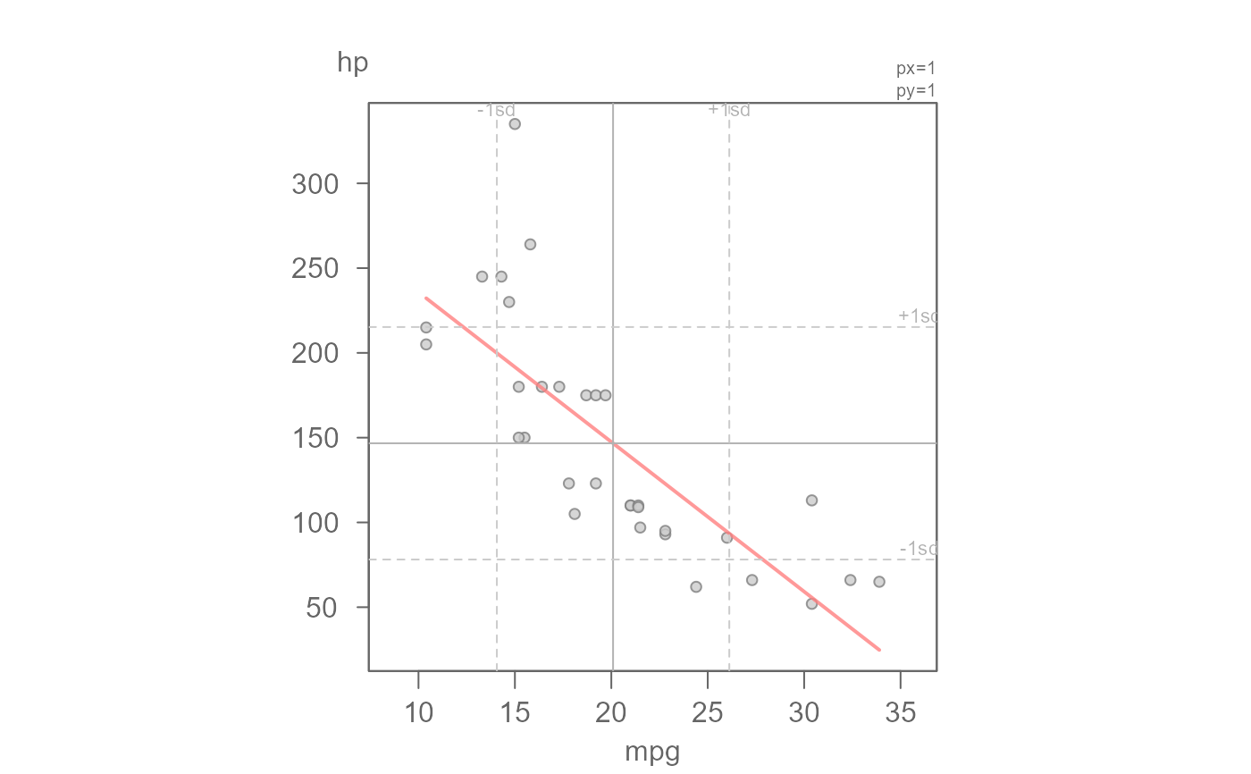
M1 <- lm(hp ~ mpg, mtcars)
eda_rfs(M1,q =TRUE)
#> The mid 90.0% of residuals covers about 112.42 units.
#> The fitted values cover a range of 207.50 units, or about 184.6% of the mid 90.0% of residuals.


M2 <- eda_lm(mtcars, mpg, hp)

#>        int      mpg^1 
#> 324.082314  -8.829731 
eda_rfs(M2,q =TRUE)
#> The mid 90.0% of residuals covers about 112.42 units.
#> The fitted values cover a range of 207.50 units, or about 184.6% of the mid 90.0% of residuals.


M3 <- eda_rline(mtcars, mpg, hp)
eda_rfs(M3, q =TRUE)
#> The mid 90.0% of residuals covers about 122.52 units.
#> The fitted values cover a range of 252.28 units, or about 205.9% of the mid 90.0% of residuals.