Simulate data using Fleishman transformation

Generates random data with the specified skewness and excess kurtosis using the Fleishman transformation method.

Usage

eda_sim(
  n = 1,
  skew = 0,
  kurt = NULL,
  check = TRUE,
  coefout = FALSE,
  coefin = NULL
)

Arguments

n: An integer specifying the number of random data points to generate.
skew: A numeric value specifying the desired skewness of the simulated data.
kurt: A numeric value specifying the desired excess kurtosis of the simulated data. A NULL value will have the function compute the minimum kurtosis value
check: Boolean determining if the combination of skewness and kurtosis are valid.
coefout: Boolean determining if the Fleishman coefficients should be outputted instead of the simulated values.
coefin: Vector of the four coefficients to be used in Fleishman's equation. This bypasses the need to solve for the parameters.

Value

A numeric vector of simulated data points.

Details

The function uses Fleishman's polynomial transformation of the form:

$$Y = a + bX + cX^2 + dX^3$$

where a, b, c, and d are coefficients determined to approximate the specified skewness and excess kurtosis, and X is a standard normal variable. The coefficients are solved using a numerical optimization approach based on minimizing the residuals of Fleishman's equations. An excess kurtosis is defined as the kurtosis of a Normal distribution (k=3) minus 3.

References suggest that the function is valid for a skewness range of -3 to 3 and an excess kurtosis greater than -1.13168 + 1.58837 * skew ^ 2. However, the suggested cutoff fails for a skewness beyond the range -2,2 in this function's implementation of Fleishman's routine. Instead, a cutoff of -1.13168 + 0.9 + 1.58837 * skew ^ 2 is implemented here.

If check = TRUE, the function will warn the user if an invalid combination of skewness and excess kurtosis are passed to the function. If kurt = NULL , the function will generate the minimum valid excess kurtosis value given the input skewness.

If the proper combination of skewness and kurtosis parameters are passed to the function, the output distribution will have a mean of around 0 and a variance of around 1. But note that a strongly skewed distribution will require a large n to reflect the desired properties due to the disproportionate influence of the tail's extreme values on the various moments of the distribution, particularly higher-order moments like skewness and kurtosis.

Fleishman, A. I. (1978). A method for simulating non-normal distributions. Psychometrika, 43, 521–532.
Wicklin, R. (2013). Simulating Data with SAS (Appendix D: Functions for Simulating Data by Using Fleishman’s Transformation). Cary, NC: SAS Institute Inc. Retrieved from https://tinyurl.com/4tustnph

Examples


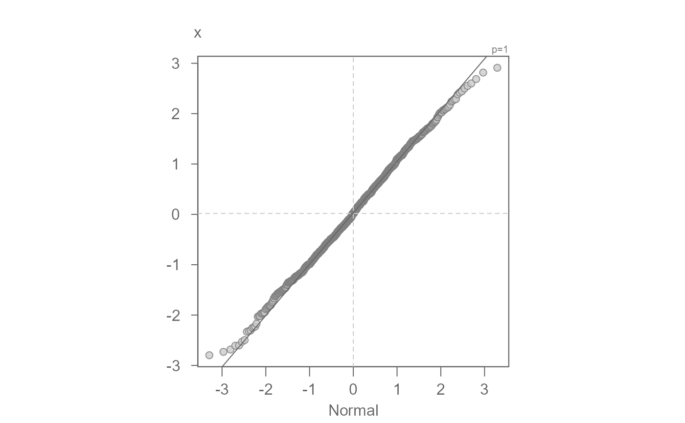
# Generate a normal distribution
set.seed(321)
x <- eda_sim(1000, skew = 0, kurt = 0)
#> Skew/kurtosis combination is valid.
eda_theo(x) # Check for normality


# Simulate distribution with skewness = 1.15 and kurtosis = 2
# A larger sample size is more likely to reflect the desired parameters
set.seed(653)
x <- eda_sim(500000, skew = 1.15, kurt = 2)
#> Skew/kurtosis combination is valid.

# Verify skewness and excess kurtosis of the simulated data
# Mean and variance should be close to 0 and 1 respectively
eda_moments(x)
#>             n          mean           var          skew          kurt 
#>  5.000000e+05 -4.100630e-04  9.991292e-01  1.159680e+00  2.085365e+00 

# Visualize the simulated data
hist(x, breaks = 30, main = "Simulated Data", xlab = "Value")


# Check skewness/kurtosis output
set.seed(123)
skew <- kurt <- z <- vector()
y <- seq(-3.5,3.5, by = 0.5)
for (i in 1:length(y)){
 z[i] <- -1.13168 + 0.9 + 1.58837 * y[i]^2 # Compute within range kurtosis
 x <- eda_sim(199999, skew = y[i], kurt = z[i], check = FALSE)
 skew[i] <- eda_moments(x)[4]
 kurt[i] <- eda_moments(x)[5]
}

eda_qq(y, skew)

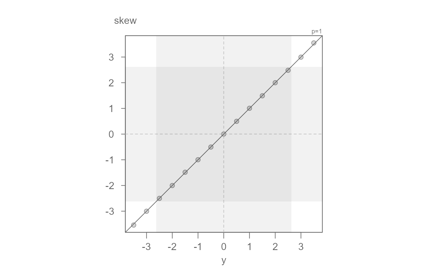#> [1] "Suggested offsets:y = x * 0.9996 + (-0.0027)"
eda_qq(z,kurt)

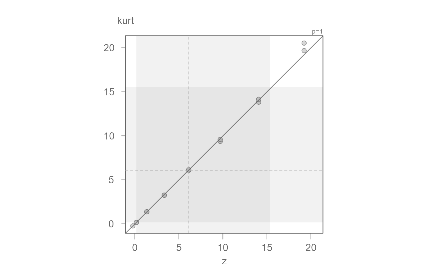#> [1] "Suggested offsets:y = x * 0.9998 + (-0.0042)"