| ggplot2 | tukeyedar |
|---|---|
| 4.0.2 | 0.5.0 |
32 Parameterizing the Residuals
In the univariate section of this course, we learned that parameterizing residuals offers many benefits, including the ability to succinctly characterize spread using a single parameter, such as the standard deviation. While the standard deviation is broadly applicable, it is most commonly associated with the Normal distribution. This association arises because, in many statistical methods and contexts (e.g., hypothesis testing and confidence intervals), the assumption of Normality in the residuals simplifies analysis. In this context, we assume that \(\epsilon_i \sim N(0, \sigma^2)\) meaning that each residual \(\epsilon_i\) is independently and identically distributed according to a Normal distribution with a mean of 0 and a constant variance \(\sigma^2\).
32.1 Checking residuals for normality
If you plan to conduct a hypothesis test (e.g., testing whether the slope is significantly different from 0), it is important to check whether the residuals are approximately Normal since this is an assumption made when computing a confidence interval and a p-value.
We learned that a Normal quantile-quantile plot was well suited for this comparison. For example, using the eda_theo function, we can compare the model’s residuals to a unit Normal distribution.
library(tukeyedar)

M <- lm(mpg ~ hp + I(hp^2), mtcars)
residuals <- M$residuals
eda_theo(residuals)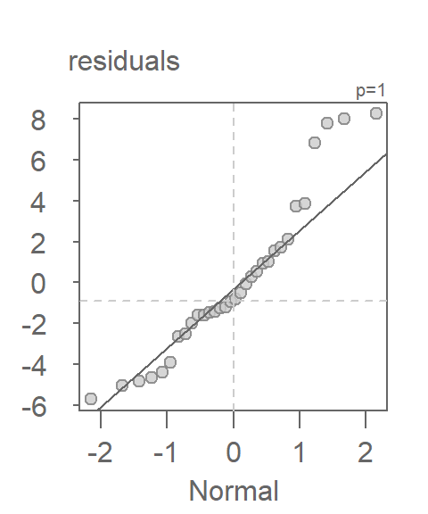
You can also generate the same theoretical QQ plot using ggplot2 with the stat_qq() and stat_qq_line() functions.
library(ggplot2)

ggplot() + aes(sample = residuals) +
   stat_qq(distribution = qnorm) +
   stat_qq_line(distribution = qnorm, col = "blue") +
   xlab("Normal") + ylab("Residuals")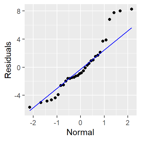
32.2 Interpreting the theoretical Q-Q plot
In a Normal Q-Q plot, residuals that follow a Normal distribution will fall approximately along the reference line. Systematic deviations from this line can indicate:
- Curvature: Suggests skewness in the residuals.
- Heavy tails: Points at the ends deviate sharply, indicating outliers or excess kurtosis.
- S-shaped patterns: May indicate a need for transformation.
32.2.1 What to do if residuals aren’t Normal
If residuals show strong departures from Normality, consider the following options:
- Transform the response variable: Common transformations include logarithmic, square root, or Box-Cox.
- Use robust regression methods: These methods are less sensitive to non-Normal residuals.
- Apply nonparametric techniques: These do not rely on distributional assumptions and can provide valid inference under broader conditions.