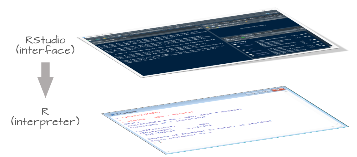
R1 and RStudio2 are are two distinct applications that serve different purposes. R is the core software that executes commands and performs computations. It’s the workhorse. Without R installed on your computer or server, you wouldn’t be able to run any commands.
RStudio, on the other hand, is an Integrated Development Environment (IDE) designed to enhance your experience with R. It provides a user-friendly interface with features like syntax highlighting, debugging tools, and visualization capabilities—making R more accessible and efficient to use.
RStudio comes in two flavors:
A desktop application that installs directly on your computer;
A server application that is accessible via a web browser.
Both platforms offer nearly identical experiences. The former runs on top of R installed on your computer, the latter runs off of an instance of R running on a remote server.
2.1.1 Do I need RStudio to interface with R?
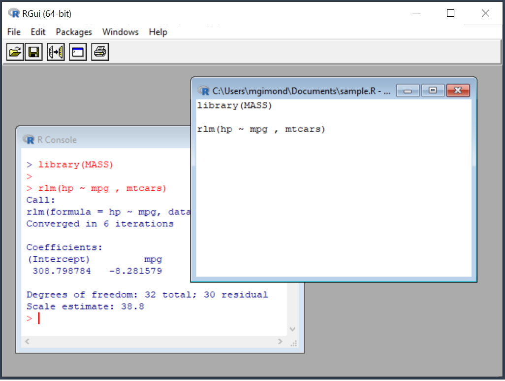
The answer is No! Many new users to the R environment conflate R with RStudio. R has been around for decades, long before RStudio was developed. In fact, when you install R on your Windows or Mac computer, you are offered a perfectly functional barebones IDE for R.
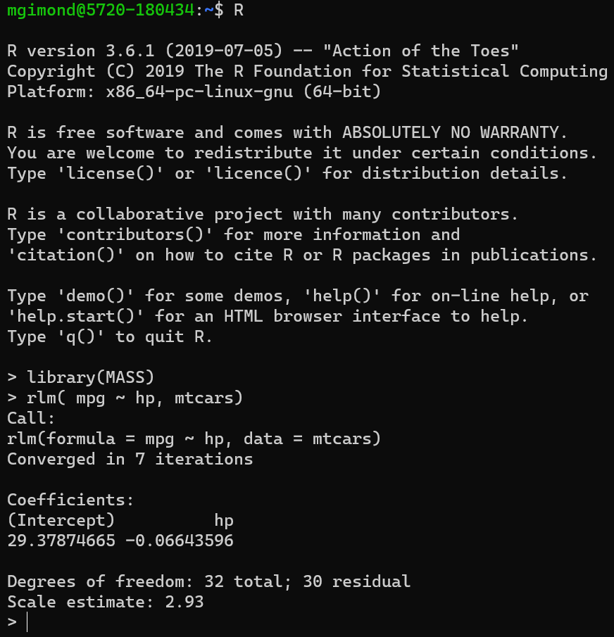
R can even be run in a shell environment like Linux:
Note that while you do not need RStudio to run R on your computer, the reverse cannot be said. In other words, RStudio is not functional without an installation of R. You therefore need to install R regardless of whether or not you use RStudio.
2.1.2 Which software do I cite?
You will normally cite R and not RStudio since RStudio does not contribute to the execution of the code (i.e. an R script will run independently of the version of RStudio or of any other IDE used to interface with R).
You can access citation information for R via:
citation()
To cite R in publications use:

  R Core Team (2025). _R: A Language and Environment for Statistical Computing_. R Foundation for
  Statistical Computing, Vienna, Austria. <https://www.R-project.org/>.

A BibTeX entry for LaTeX users is

  @Manual{,
    title = {R: A Language and Environment for Statistical Computing},
    author = {{R Core Team}},
    organization = {R Foundation for Statistical Computing},
    address = {Vienna, Austria},
    year = {2025},
    url = {https://www.R-project.org/},
  }

We have invested a lot of time and effort in creating R, please cite it when using it for data analysis.
See also 'citation("pkgname")' for citing R packages.
2.2 Command line vs. script file
2.2.1 Command line
R can be run from a R console or RStudio command line environment. For example, we can assign four numbers to the object x then have R read out the values stored in x:
x <-c(1,2,3,4)x
[1] 1 2 3 4
2.2.2 R script files
If you intend on typing more than a few lines of code in a command prompt environment, or if you wish to save a series of commands as part of a project’s analysis, it is probably best that you write and store the commands in an R script file. Such a file is usually saved with a .R extension.
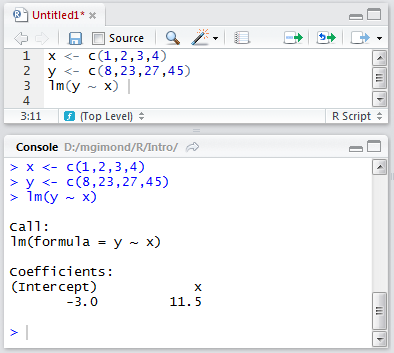
In RStudio, you can run a line of code in a R script file by placing a cursor anywhere on that line (while being careful not to highlight any subset of that line) and pressing the shortcut keys Ctrl+Enter on a Windows keyboard or Command+Enter on a Mac.
You can also run an entire block of code by selecting all lines to be run, then pressing the shortcut keys Ctrl+Enter/Command+Enter. Alternatively, you can run the entire R script by pressing Ctrl+Alt+R in Windows or Command+Option+R on a Mac.
In the following example, the R script file has three lines of code: two assignment operations and one regression analysis. The lines are run one at a time using the Ctrl+Enter keys and the output is displayed in the console window.
2.3 The assignment operator <-
When assigning values or output from operations to a variable, the assignment operator, <-, is placed between the variable name and the value(s) being assigned to that variable. In the preceding example, the values 1,2,3,4 were being assigned to x. The assignment operator is constructed by combining the less then character, <, with the dash character, -. Given that the assignment operator will be used frequently in an R script, it may be worthwhile to learn its shortcut: Alt+- on Windows and Option + - on a Mac.
Note that, in most cases, you can also use the = to assign values as in:
x = c(1,2,3,4)
However, this option is not widely adopted in the R community. An advantage in using <- instead of = is in readability. The <- operator makes it easier to spot assignments during a quick visual scan of an R script, more so than the = operator which is also used in functions when assigning parameters to function variables aas in,
M <- lm(y ~ x, data = dat, weights = wt)
The alternative would be:
M = lm(y ~ x, data = dat, weights = wt)
Notice how the assignment of M does not stand out as well in the second example given the recurrence of = on the same line of code (unless, of course, you benefit from colored syntax).
2.4 Understanding directory structures
Because a data file may reside in a different directory than that which houses the R script calling it, you need to explicitly instruct R on how to access that file from the R session’s working directory.
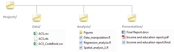
In the example that follows, user Jdoe has a project folder called Project1 in which resides a ./Data folder and an ./Analysis folder.
He opens the R script called Data_manipulation.R located in the Analysis folder. The script contains the following line of code:
dat <-read.csv("ACS.csv")
He executes that line of code and R returns the following error message:
Error in `file()`:
! cannot open the connection
The error message states that the file ACS.csv cannot be found. This is because the session’s working directory is probably set to a directory other than the D:/Jdoe/Project1/Data directory which houses the data file. An R session’s working directory can be verified by typing the following command:
getwd()
[1] "D:/jdoe/Project1/Analysis"
The working directory is used to instruct R where to look for a file (or where to create one) if the directory path is not explicitly defined. So, in the above example, user Jdoe is asking R to open the file ACS.csv without explicitly telling R in which directory to look, so R is defaulting to the current working directory which is D:/jdoe/Project1/Analysis.
There are two options to resolving this problem. The first is to set the working directory to the folder that contains the ACS.csv file using the setwd() function.
setwd("D:/Jdoe/Project1/Data")
The second is to modify the read.csv call by specifying the path to the ACS.csv file.
dat <-read.csv("D:/Jdoe/Project1/Data/ACS.csv")
However, this approach makes it difficult to share the project folder with someone else who may choose to place the project folder under a different folder such as C:\User\John\Documents\Project1\. In such a scenario, the user would need to modify every R script that references the directory D:\Jdoe\Project1\. A better solution is to specify the location of the data folder relative to the location of the Analysis folder such as,
dat <-read.csv("../Data/ACS.csv")
The two dots, .., tells R to move up the directory hierarchy relative to the current working directory. In our working example, ../ tells R to move out of the Analysis/ folder and up into the Project1/ folder. The relative path ../Data/ACS.csv tells R to move out of the Analysis/ directory and over into the Data/ directory before attempting to read the contents of the ACS.csv data file.
Using relative paths makes your project folder independent of the full directory structure in which it resides thus facilitating the reproducibility of your work on a different computer or a different root directory environment. This assumes, of course, that the user will set the working directory to the project folder location.
2.5 Packages
One of R’s attractive features is its rich collection of packages that facilitate collaborative research by enabling the sharing of functions, data, and methodologies among scientists and researchers. While some packages are pre-installed with R, many others can be easily accessed and installed from repositories like CRAN, GitHub, or even individual websites.
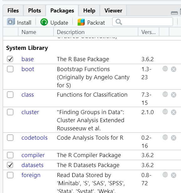
2.5.1 Base packages
R comes installed with a set of default packages. A snapshot of a subset of the installed base packages is shown below:
2.6 Installing packages from CRAN
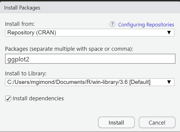
Many packages can be installed from the CRAN repository. To install a CRAN package from within RStudio, click on the Packages tab, select Install and choose Repository (CRAN) as the source location. In the following example, the library ggplot2 is installed from CRAN.
Package installation from CRAN’s repository can also be accomplished by typing the following line of code in a console:
install.packages("ggplot2")
The installation process is typically straightforward. If dependencies are encountered (i.e. other packages required by the primary package), R will automatically install them as long as the Install dependencies option is selected. For example, ggplot2 relies on several supporting packages, such as RColorBrewer and reshape2, which are automatically installed alongside it.
R packages are typically installed within the user’s home directory by default. This offers the advantage of not requiring administrative privileges on the computer. However, this can also be a limitation. If another user logs in on the same machine, they will not have access to the packages you’ve installed and will need to install them separately in their own home directory, potentially leading to multiple copies of the same package on the system.
2.6.1 Installing packages from GitHub
Some packages may be in development and deemed not mature enough to reside on the CRAN repository. Such packages are often found on GitHub–a website that hosts software projects. Installing a package from GitHub requires the use of another package called remotes available on CRAN.
For example, to install the latest version of ggplot2 from GitHub (i.e. the developmental version and not the stable version available on CRAN) type the following:
install.packages("remotes") # Install the remotes package (if not already present)library(remotes) # Load the remotes package in the current R sessioninstall_github("tidyverse/ggplot2")
The argument tidyverse points to the name of the repository and ggplot2 to the name of the package.
2.6.2 Using a package in a R session
Installing an R package on your computer does not automatically make its functions available for immediate use within an R session. You must explicitly load the package into your current R session before you can use its functions.
For example, after installing the ggplot2 package, you might want to use one of its functions, ggplot, to generate a scatter plot,
ggplot(mtcars, aes(mpg, wt)) +geom_point()
only to see the following error message:
This is because ggplot2 package have not been loaded into the current R session. To make its functions and/or data available in an R session, you must load its content using the library() function:
library(ggplot2)
Once the package is loaded in the current R session, you should have full access to its functions and datasets.
ggplot(mtcars, aes(mpg, wt)) +geom_point()
2.7 Getting a session’s info
To ensure the transparency of your analyses, it’s important to document all aspects of your analytical environment alongside your data and results. This includes the specific versions of R and all key packages used. This is essential because the behavior of functions and environments can change across versions, either intentionally through updates or unintentionally due to bug fixes. No software, regardless of its origin, is exempt from such changes. To facilitate this documentation, simply call the sessionInfo() to capture a snapshot of your current R session, including the installed packages and their versions.
Here’s an example of a session’s R environment:
sessionInfo()
R version 4.5.2 (2025-10-31 ucrt)
Platform: x86_64-w64-mingw32/x64
Running under: Windows 11 x64 (build 26100)

Matrix products: default
  LAPACK version 3.12.1

locale:
[1] LC_COLLATE=English_United States.utf8  LC_CTYPE=English_United States.utf8    LC_MONETARY=English_United States.utf8
[4] LC_NUMERIC=C                           LC_TIME=English_United States.utf8

time zone: America/New_York
tzcode source: internal

attached base packages:
[1] stats     graphics  grDevices utils     datasets  methods   base

other attached packages:
[1] ggplot2_4.0.2

loaded via a namespace (and not attached):
 [1] vctrs_0.7.1        cli_3.6.5          knitr_1.51         rlang_1.1.7        xfun_0.56          otel_0.2.0
 [7] generics_0.1.4     S7_0.2.1           jsonlite_2.0.0     labeling_0.4.3     glue_1.8.0         htmltools_0.5.9
[13] scales_1.4.0       rmarkdown_2.30     grid_4.5.2         tibble_3.3.1       evaluate_1.0.5     fastmap_1.2.0
[19] lifecycle_1.0.5    compiler_4.5.2     dplyr_1.2.0        codetools_0.2-20   RColorBrewer_1.1-3 pkgconfig_2.0.3
[25] htmlwidgets_1.6.4  rstudioapi_0.18.0  farver_2.1.2       digest_0.6.39      R6_2.6.1           tidyselect_1.2.1
[31] pillar_1.11.1      magrittr_2.0.4     withr_3.0.2        tools_4.5.2        gtable_0.3.6
R Core Team (2020). R: A language and environment for statistical computing. R Foundation for Statistical Computing, Vienna, Austria. URL https://www.R-project.org/↩︎
RStudio Team (2021). RStudio: Integrated Development for R. RStudio, PBC, Boston, MA URL http://www.rstudio.com/.↩︎